Physics based Motion Estimation to Improve Video Compression

James McCullough

, Naseer Al-Jawad

and Tuan Nguyen

School of Computing, University of Buckingham, Hunter Street, Buckingham, U.K.

School of Computing & Mathematical Sciences, University of Greenwich, Old Royal Naval College, Park Row, London, U.K.

Keywords: Video Compression, Optical Flow, Physics, Mechanics, Acceleration, Velocity, Segmentation.

Abstract: Optical flow is a fundamental component of video compression as it can be used to effectively compress

sequential frames. However, currently optical flow is only a transformation of one frame into another. This

paper considers the possibility of representing optical flow based on physics principles which has not, to our

knowledge, been researched before. Video often consists of real-world events captured by a camera, meaning

that objects within videos follow Newtonian physics, so the video can be compressed by converting the motion

of the object into physics-based motion paths. The proposed algorithm converts an object’s location over a

series of frames into a sequence of physics motion paths. The space cost in saving these motion paths could

be considerably smaller compared with traditional optical flow, and this improves video compression in

exchange for increased encoding/decoding times. Based on our experimental implementation, motion paths

can be used to compress the motion of objects on basic trajectories. By comparing the file sizes between

original and processed image sequences, effective compression on basic object movements can be identified.

1 INTRODUCTION

The goal of video compression is to minimise the size

of digital video files. This area has been studied

extensively, focusing on compressing the data in

several different ways, which can be divided into two

categories: intra-frame and inter-frame compression.

Intra-frame compression is applied within individual

frames without concern of surrounding frames; this is

equivalent to regular image compression. Inter-frame

compression, however, focuses on how similar

consecutive frames can be compressed, such as

saving vectors to transform one frame into the next if

the two are similar enough to achieve this. However,

given a large quantity of video produced contains

objects from real life, it may be possible to

retroactively apply physics movement to objects

captured on camera. The aim of this paper is to

propose a method to transform object motion into

physics-based motion paths which can be used to

compress this information.

Currently available methods for video

compression are inbuilt into video codecs (the

https://orcid.org/0000-0002-8422-0347

https://orcid.org/0000-0002-4585-6385

https://orcid.org/0000-0003-0055-8218

formats for how video is stored on digital devices)

such as H.264 and HEVC (also called H.265) which

are the two most adopted at the time of writing. Both

example codecs use optical flow / motion estimation

to generate motion vector arrays to trace the

movement of groups of pixels (termed micro

blocks/coding tree units) from one frame to another.

To clarify, motion estimation is the term relating to

estimating motion in the world, whereas optical flow

refers specifically to estimating motion of pixels with

the video frame (Sellent et al., 2012). These two are

not always equal, but in most cases are. This allows

them to compress the information by storing the pixel

values of only one frame and then only the motion

vectors used to transform that frame to the next;

however, this process is only ever used to convert one

frame to another. This paper proposes the possibility

of using physics to transform these individual motion

vector arrays into motion paths defined by physics

principles, thus adding an additional layer onto the

already existing compression.

As this concept is in its early stages, the

experimental setup applies physics to the movement

of individual segmented objects from the DAVIS

364

McCullough, J., Al-Jawad, N. and Nguyen, T.

Physics based Motion Estimation to Improve Video Compression.

DOI: 10.5220/0010811900003124

In Proceedings of the 17th International Joint Conference on Computer Vision, Imaging and Computer Graphics Theory and Applications (VISIGRAPP 2022) - Volume 4: VISAPP, pages

364-371

ISBN: 978-989-758-555-5; ISSN: 2184-4321

2016 dataset (Perazzi et al., 2016). Then, the file sizes

of the original image sequence can be compared with

the extracted object and background sequences along

with the new generated physics motion path data.

Video compression is a beneficial field of study as

video is stored digitally almost exclusively. At high

resolutions such as 4K, reducing the file sizes should

enable faster video file transfers, and reduce hardware

and energy costs. The aim is that applying physics to

object motion within videos would allow increased

compression rates and a new branch of potential

research is discovered.

2 LITERATURE REVIEW

There is, to the author’s knowledge, no current

research into using physics to improve video

compression, so this research focuses on relevant

existing video compression methods that could be

used as a base to build on. Optical flow is a key

component in video compression, and there are a

wide variety of different approaches and methods

available to calculate it. One key method is block

matching/motion blocking, which is compared with

other methods by Philip et al. (2014). Optical flow is

saved in the form of a motion vector array, which is a

transformation from one frame into another, and this

makes it a possible input for our proposed physics

estimation algorithm. Each frame’s optical flow

encodes the translation of all applicable pixels within

the video, which can be further compressed using

physics-based motion paths in our proposed method.

Further research was carried out on the variety of

different optical flow methods (Barron et al., 1994),

and more specifically using segmentation with optical

flow as the objects would need to be extracted from

the videos. DeepFlow (Weinzaepfel et al., 2013)

effectively adapted optical flow to handle larger

displacements, while ObjectFlow (Tsai et al., 2016)

builds on it and other similar methods to use optical

flow to segment objects and would be useful as a

segmentation process before physics estimation.

Currently, the two most commonly used codecs

(H.264, H.265) each use a version of motion blocking

to generate the optical flow used, with the only

difference being the sizes of the motion blocks used,

and thus the number of motion vectors stored

(Rajabai & Sivanantham, 2018). Our proposed

method is to build upon the output of these created

motion vectors to apply physics estimation to their

movement throughout the video.

Many related studies were included within the

research involving components of optical flow and

segmentation in order to inform this study. Tsai et al.

(2016) uses optical flow to discern object boundaries

which would be a useful basis to then apply physics

to. Motion Blocking also could be expanded upon, for

example Gao et al. (2020) develops upon the method

by breaking down motion blocks into a large number

of possible polygons. This resulted in 82 options,

which allowed motion blocks to be divided

effectively along object edges. By improving the

accuracy of how motion blocks represent objects, this

would allow for semi-segmentation within the motion

blocking process and the proposed physics process

could then be applied more effectively. Being able to

detect and recognise camera movements will also be

important for adjusting the axis that the physics is

measured against, so authors such as Sandula &

Okade (2019) suggesting methods of detecting such

camera movements were also researched. These

issues could also be corrected with some inversion of

motion stabilization where the axis measured against

is stabilized to the camera movement. This can also

be achieved during the motion blocking stage of

compression (Wang et al., 2017), which analyses the

global motion parameters to stabilize the video.

To keep it simple for this proof-of-concept, we

use a segmented dataset and track object movement

via its centre point without regarding any rotation or

other transformation. These will be areas that require

more investigation if this proof-of-concept indicates

a value to physics-based compression.

While physics/mechanics has been widely

explored in areas such as computer vision and object

tracking, the authors have not seen any examples of

an attempt to implement it into video compression.

3 METHODOLOGY

This paper aims to build a process that can compress

videos by segmenting each video frame into objects,

and then analysing the object’s motion in terms of

physics equations which allows this motion data to be

compressed. Firstly, the paper will outline some

physics concepts, then these will be used to convert

object location data into motion paths based on these

concepts, and finally this will be implemented into a

basic video compression process.

As this is a proof-of-concept, this paper is solely

concerned with a physics-based representation of

motion. This means rotation, scaling and

complex/non-rigid objects are disregarded at present.

We also use a segmented dataset to perform an

intuitive test without needing to solve the complicated

issues behind object tracking, but do not suggest

Physics based Motion Estimation to Improve Video Compression

365

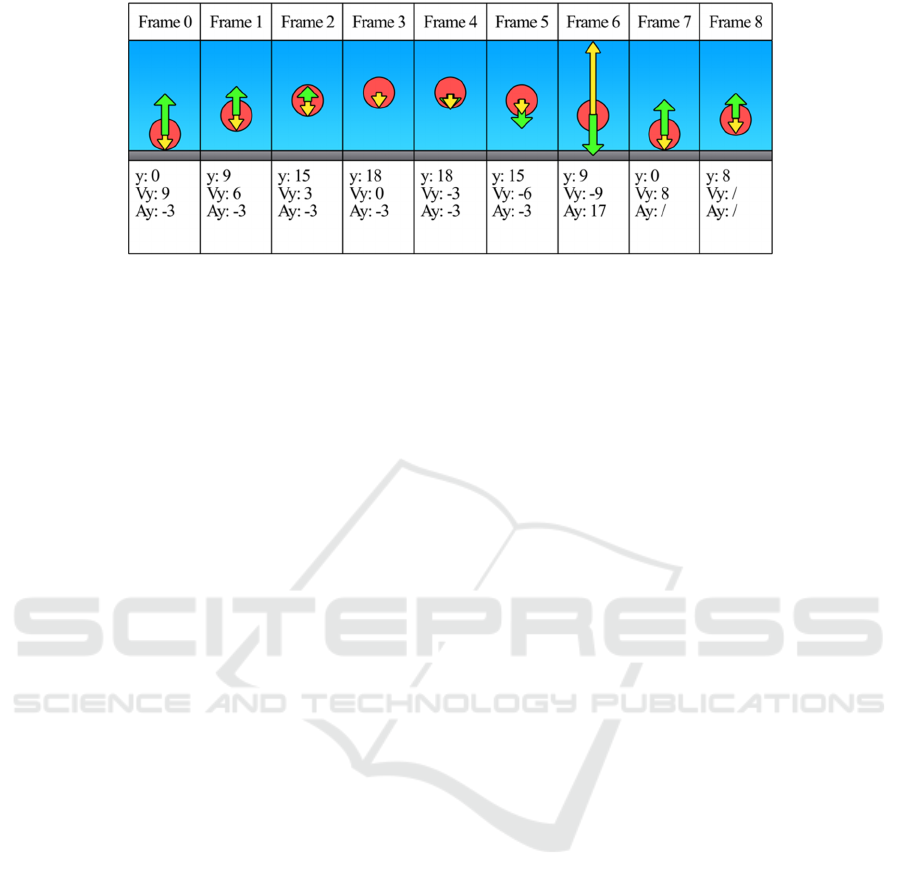
Figure 1: A conceptual video sequence of a ball bouncing with the calculated values of location (y), velocity (Vy) and

acceleration (Ay) for each frame. The values for Vy and Ay are calculated using Equations (1) & (2). The arrows are visual

representations of the velocity (green) and acceleration (yellow). For simplicity, only the y dimension is specified.

segmentation as a method for tracking objects in

future as it is a more intensive process than video

compression requires.

3.1 Physics Concepts

To explain our proposed video compression

technique, it is important to first outline the basic

physics concepts used to achieve it. All object

interactions can be modelled by many different

physics frameworks. For example, the theory of

relatively could be used (Einstein, 2010), but this was

created to update the previous framework’s

interpretation of particles interacting in extreme cases

(such as close to light speed). Newtonian physics

however is what is more typically used to simulate

object interactions at the time of writing, and it is

more mathematically simple to model. As such,

Newtonian physics will be used to build this

modelling of object movement.

Movement in Newtonian physics relies on the

basic concepts of location, velocity and acceleration.

Location is the place where an object is, at a set time

or frame. Velocity is the difference between the

location of the object over a set gap in time (for video

purposes, one frame to the next). Acceleration is the

difference between the velocity of an object at one

point in time, and the velocity of an object at the next

point in time. For an object in motion while no new

force acts upon it, the object’s acceleration will

remain constant, manipulating its velocity which in

turn influences its location (Raine, 2013). These

concepts are formalised in equations (1) and (2)

below, which are then demonstrated visually in

Figure 1. Newtonian Physics concepts can be

demonstrated more clearly using Figure 1, which is a

ball bouncing sequence accompanied by values for its

distance, velocity and acceleration, as would be

calculated using the definitions of location, velocity

and acceleration stated.



𝑉𝑥



,𝑉𝑦







𝑥



𝑥



,𝑦



𝑦





(1)



𝐴

𝑥



𝐴

𝑦







𝑉𝑥



𝑉𝑥



,𝑉𝑦



𝑉𝑦





(2)

where [x

, y

] is the object’s location within frame n

For simplicity, the y values are measured as the

distance from the ground, however in implementation

they are calculated vertically from the top of the

frame. Figure 1 demonstrates this Newtonian physics

concept as acceleration remains constant as the ball

bounces, until it impacts with the ground on frame 7

where the ball’s gravitational force is combined with

the impulse force from the ground causing the ball’s

acceleration to spike in the other direction for a single

frame. Because of the discrete nature of frame by

frame video, this acceleration is observed on frame 6

because of the large change in velocity.

This approach may seem over-simplified given

that there appear to be many forces acting upon the

ball over time. For example, the ball is affected by the

force of gravity permanently pulling it downwards,

and an occasional impulse force from the ground.

However, this method calculates the acceleration

from the movement of the ball, and as such does not

need to concern itself with the individual forces. Any

combination of forces creates a set acceleration for as

long as those forces continue to act on the object, and

as the process can calculate the acceleration from the

observed movement, individual forces are catered for.

This indicates that no matter the object or the

motion, be it a boat sailing along a river or clouds

moving across the sky, the motion of any object can

be simplified into only the acceleration, velocity and

location of the object over a sequence of frames.

VISAPP 2022 - 17th International Conference on Computer Vision Theory and Applications

366

3.2 Optical Flow into Motion Paths

Optical flow is the vector array to transform one

frame into the next. Finding optical flow is a complex

task. There are many differing methods, along with

numerous extensions, to calculate optical flow.

Our proposed method is that the optical flow field

has some underlying redundancy which can be

extracted through the process of physics modelling,

allowing for further compression. Because the optical

flow field is representative of object movements

between only two frames, considering a series of

optical flow frames together, it is likely possible to

group objects together and apply physics to model the

object movements. This is because the motion of

objects does not vary randomly between each frame,

but instead follows a defined path in relation to the

object’s movement in the world. As such, it should be

possible to save optical flow data in the form of

physics equations, and this may have a smaller file

size than the optical flow data itself. This is quite a

complex problem, especially transforming an optical

flow field into distinct objects and maintaining their

persistence throughout a video sequence. This kind of

segmentation has been studied before (Kim et al.,

2003, p. 2; Kung et al., 1996) and indicates that the

proposed method has potential. For example, if

vectors of a similar direction and amplitude can be

clustered together, objects within the video should be

determinable. The same objects movements over the

course of multiple frames can then be converted into

physics motion paths.

Figure 2: Optical flow field example.

Figure 2 shows a depiction of optical flow where the

frame is broken down into blocks, and the arrows

represented the how the pixels are transformed from

one frame into the next. The vast majority of pixels

shift only a small amount, but there are a number of

outlier vectors that have been mismatched with a

similar but different section of the image.

However, the conversion of this optical flow data

into objects is quite a complex problem, so it would

be sensible to determine if saving data into a motion

path format will improve the compression ratio before

attempting to solve it. As such, this paper proposes a

simple proof-of-concept test using pre-segmented

video to extract object coordinates, from which to

determine object motion.

3.3 Converting Filmed Object

Coordinates into Motion Paths

To achieve the video compression, a process has been

constructed to transform a series of coordinates into

motion paths based on physics. This process is

outlined in the flow chart in Figure 3. The input to this

flow-chart is a series of coordinates, and the output is

the corresponding series of motion paths. It is

possible to demonstrate the process with the ball

bouncing sequence from Figure 1.

To begin with, the counter n is used to count

frames through the sequence. A threshold must also

be determined to register a change in acceleration.

Given the discretisation caused by video having a

limited frame rate, a small threshold value should be

chosen to discern big jumps in acceleration, as there

will likely be minor changes detected throughout. In

this case, 1 is a suitable value. It is initialised to the

start of the sequence: frame 0. As there are more than

3 frames in the sequence, the details of that first frame

are saved as the first motion path according to

equations (1) and (2): M[y = 0, Vy = 9, Ay = -3] as

location (y), velocity (Vy) and acceleration (Ay)

respectively. The counter is now increased by 3,

because the first three frames are always accurately

represented as they were used to calculate the motion

path’s values. Then, the new frame’s acceleration is

calculated, and as it is also -3, it is within a threshold

distance from the path’s acceleration (also -3), so the

counter is increased again. This loop will continue

until the counter is equal to 6, as here the calculated

acceleration is now 17 which is outside the threshold

accepted radius around -3 (-4 to -2 are acceptable for

a threshold of 1), so this concludes that motion path.

As there are no longer 3 frames remaining, but only

2, a dummy motion path is generated with no

acceleration to store the location information for the

final two frames, and the process is completed.

In order to generate the original coordinates back

from these motion paths, the following function can

be used.

𝑀





𝑗



=

𝑘,

𝑗

𝑀



𝑗

1



+𝑉𝑘,

𝑗

𝑀



𝑗

1



+𝑉𝑘+



𝑗

1



𝐴𝑘,

𝑗

1

(3)

where j = n – m for a path starting at frame m and n

is the frame in the sequence, and k is x and y,

performed on the [x, y] vector.

Physics based Motion Estimation to Improve Video Compression

367

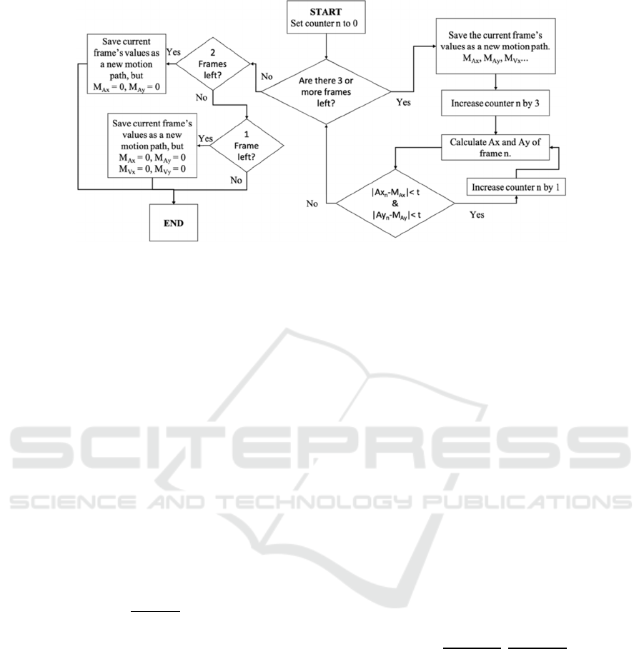
Figure 3: A flowchart showing the coordinate to motion path process, where Ax

is the acceleration on frame n in the x axis,

and M

is the acceleration of the current motion path in the x axis, and so forth.

For example, to gain the value from frame 3 using

the saved motion paths, j = 3 as the motion path

begins at frame 0, the function can then be solved

recursively for M

(3).

The remaining issue is how to determine the

threshold value that detects a change in acceleration

effectively. The value of 1 works for the example, but

from sequence to sequence the optimum threshold is

likely to change. If the threshold is set too low, then

motion paths will be unnecessarily created which will

negate compression. If the threshold is too high, then

the object will veer off its intended path because a

new path is not created when it should be.

𝐹



𝑛



=

𝑥



𝑀





𝑛

|

𝑡 ∩ 𝑦



𝑀





𝑛



𝑡

0, 𝑂𝑡ℎ𝑒𝑟𝑤𝑖𝑠𝑒

(4)

where [x,y] is the object’s location, t is a tolerance

and M is the function specified in (3)

𝐴

∑









(5)

where N is the total number of frames in the sequence

To solve this issue, a function is proposed defined

in equations (4) and (5) to test every frame. Equation

(5) returns a percentage of frames where the object’s

location has been placed correctly by the algorithm,

using a small value for t to allow for acceptable

displacement. This displacement of the object within

the image is the only change to video quality

introduced by the proposed method, and while this

can be set to 0 to ensure no change/lossless

compression, this would also limit the compression

achievable. The target accuracy can now be set to 1

to ensure the algorithm’s recreations do not vary from

the true locations of the objects and the process could

then be run repeatedly to generate and test object

paths while shifting the threshold up and down until

A = 1 . This method allows for some variation in

acceleration so long as the motion path tracks the

object accurately.

3.4 Video Compression using Physics

Paths

Here is a proposed test to determine the effectiveness

of the process discussed in section 3.3. While physics

motion paths should eventually be implemented on

top of current optical flow methods, it was decided to

keep these initial proof-of-concept tests simple by

using a segmented dataset to extract the object from

each frame and track its motion. Figure 4 shows the

encoding process. Each video sequence contains one

segmented object of focus. This object is extracted

from the background image for each frame and a list

of the object’s centre points is generated using the

centre point, described in equation (6).

𝐶



𝑥,𝑦



=























(6)

Where x

max

is the largest x coordinate within the

object, x

min

is the smallest x coordinate within the

object, y

max

is the largest y coordinate within the

object and, y

min

is the smallest y coordinate within the

object.

These centre points are then passed into the

previously discussed physics estimation function

specified in section 3.3 and then the resulting motion

paths, as well as the background and object image

sequences are saved into an encoded file. For a single

object video, this file will consist of a background

plate, an object sequence and the motion paths for the

object. For multiple-object videos, the file will consist

VISAPP 2022 - 17th International Conference on Computer Vision Theory and Applications

368

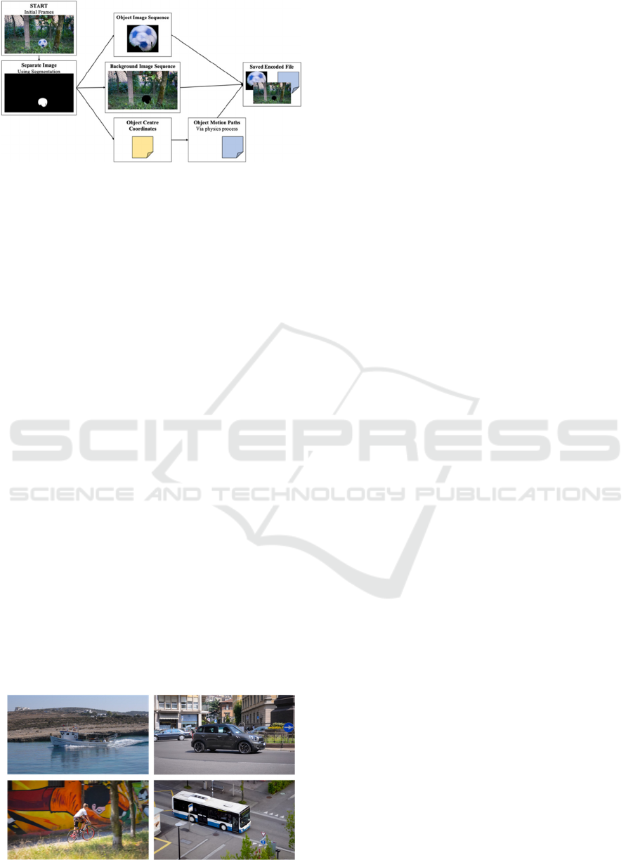
Figure 4: A flowchart breaking down the video.

of a background plate and several object sequences

each with their own motion paths. Each motion path

consists of three vectors, one for initial location, one

for initial velocity and one for acceleration; an object

may have many of these throughout the sequence. To

decode, the object need only be added to the

background frame at the coordinate retrieved from the

motion path, which is very easy to read consecutively

because of the recursive nature of equation (3). A

possible implementation could be: at the start of each

motion path, load the values of location, velocity and

acceleration into some temporary variables; then for

each frame add the velocity to the location; and add

the acceleration to the velocity; repeat this until the

start of the next motion path where the variables are

overwritten, and this process can continue being

repeated until the end of the image sequence.

4 EXPERIMENTATION AND

RESULTS

4.1 Dataset

This process has been tested using a pre-segmented

dataset and using the coordinates set by taking the

centre of the segmented object in each frame using

equation (6). The DAVIS 2016 Dataset has been used

for the featured tests (Perazzi et al., 2016). This

Figure 5: Example frames from the DAVIS 2016 dataset.

dataset was chosen as it only segments one object per

sequence and contains a wide variety of movement

types with stationary and moving camera angles, as

well as objects overlapping and complicated

segmentation. In particular, three sequences with

simplistic motion (‘soccerball’, ‘boat’ and ‘car-

roundabout’) and three sequences with complicated

motion (‘bus’, ‘bmx-trees’ and ‘hockey’) were

selected to test. The ‘soccerball’ is the simplest

sequence in that the camera is stationary and the ball

rolling along is a smooth deceleration, although the

ball does roll behind some trees which renders the

currently implemented centre tracker inaccurate in

places. The ‘boat’ sequence has a smooth panning

camera and a boat which is not overlapped by any

objects resulting in a simple motion of the boat

moving only slightly horizontally, and ‘car-

roundabout’ also has a smooth camera and no

overlapping elements in its environment.

The ‘bus’ sequence involves the bus driving

behind several signs and a tree, where the overlap

segmentation becomes very detailed, while the

motion is simple as with the car. This sequence was

included to indicate if the complexity of the

segmentation has an effect on the file-size of the

separated images. The ‘bmx-trees’ sequence is also

complex in that the camera shakes quite considerably

and the object is also a human riding a bike, making

its motion more erratic and less consistent. Finally,

‘hockey’ was included as an example of entirely

human movement where the human and the hockey

puck are tracked together as a very complicated and

unpredictable shape moving also unpredictably. This

was included to identify how the system would

handle incorrectly segmented objects, as the human

and puck’s centre point together is not representative

of a real object’s movement.

4.2 Experiments

The current implementation is only focused on the

centre-point of these objects and tracking that point’s

movement. The tested implementation makes no

attempt to break them up into individual components,

even though they may have their own individual

motion such as the BMX bike’s wheels.

In order to test the effectiveness of the proposed

process as a compression algorithm, it was going to

be compared against H.264. The comparison would

have been the size of the raw video file in .mp4

format, against the size of the two separated video

files and the saved motion path information.

However, the results of this test were that the

background plate (with the object removed) was

Physics based Motion Estimation to Improve Video Compression

369

larger in size than the original base image for every

test. We theorise this is because the empty space is

more costly when compressed by the H.264 codec

than when the object is present in the scene.

So, instead, the size of the original frames was

compared with the size of the segmented frames and

the motion data, which has been generated using the

processes described in section 3.3. The dynamic

threshold was used for the experiment to test the

different sequences on a comparable playing ground,

with a target accuracy of 1 (see equation (5)). A target

of 1 ensures each and every frame in the sequence is

accurately represented, while ensuring the minimum

number of motion paths to enable compression.

This experiment was run in Python 3.7 using

OpenCV to read and process the images, Numpy for

matrix manipulation and Pickle for saving the motion

path data. The threshold value was initialised at 1.0

and was stepped up or down by 0.05 until the target

accuracy was reached. If the threshold was lowered to

0, then the test would proceed automatically, but this

would result in an accuracy of 1, as it is equivalent to

saving all the coordinates. The tolerance t (see

equation (4)) was set to 3 pixels, as we were unable

to identify that level of displacement with a visual

inspection of the footage.

𝑆𝑖𝑚𝑢𝑙𝑎𝑡𝑖𝑜𝑛 𝑇𝑜𝑡𝑎𝑙=𝐵𝑎𝑐𝑘𝑔𝑟𝑜𝑢𝑛𝑑 𝐼𝑚𝑎𝑔𝑒 𝑆𝑖𝑧𝑒 +

𝑂𝑏𝑗𝑒𝑐𝑡 𝐼𝑚𝑎𝑔𝑒 𝑆𝑖𝑧𝑒+ 𝑀𝑜𝑡𝑖𝑜𝑛 𝐷𝑎𝑡𝑎 𝑆𝑖𝑧𝑒

(7)

𝑃𝑒𝑟𝑐𝑒𝑛𝑡𝑎𝑔𝑒 𝐷𝑖𝑓𝑓𝑒𝑟𝑒𝑛𝑐𝑒=

𝑆𝑖𝑚𝑢𝑙𝑎𝑡𝑖𝑜𝑛 𝑇𝑜𝑡𝑎𝑙

𝐵𝑎𝑠𝑒 𝐼𝑚𝑎

𝑔

𝑒 𝑆𝑖𝑧𝑒

(8)

4.3 Results

These tests revealed a substantial amount about the

proposed process. The simplest clip ‘soccerball’

performed the best with a percentage difference of

64% in comparison to the size of original image

sequence. The ‘boat’ sequence, however, performed

less well with only a 98% percentage difference, so

only 2% smaller than the original file. The surprising

result was the ‘bmx-trees’ sequence, which had a

reduction to 74% its original file size despite the

complexity of the motion in the sequence. As

expected, the more complicated sequences performed

less well, actually expanding the file size by up to

150% of their original size for the very complicated

overlapping ‘bus’ sequence. ‘bmx-trees’ and ‘car-

roundabout’ sequences were an exception,

performing in opposition to our prediction. The

results confirmed the hypothesis that image

sequences can be compressed using motion paths.

4.4 Discussion

Results from the testing show the file size is

unfortunately affected far more by the segmented

image sizes than by the motion data. This reaffirms

that applying segmentation in this way may be more

costly than it is advantageous in many cases,

especially where overlapping causes the

segmentation to be very complex. This is also

reflected in the increase in the background size when

in video format, which could be attributed to the

background plate containing a large empty area with

no details to save and track, using motion blocking.

While the motion paths themselves appear to be

working effectively, the segmentation can greatly

increase the file size which may far outweigh the

compression advantages of the motion paths on more

complicated objects and movements. This aligns with

our initial understanding as segmentation is not

suggested to replace traditional optical flow methods.

Object size also has an effect as larger objects that

take up more of the frame have a more complex

segmentation, even without considering overlapping.

A more relevant possible contributing factor is

that video is discrete in terms of having a limited

number of frames per second, whereas these physics

Table 1: Comparing the size of the original frames of the image sequence, and the separated frames of the image sequence.

Image

Sequence

Background

Image Size

(Bytes)

Object Image

Size (Bytes)

Motion Data

Size (Bytes)

Simulation

Total (Bytes)

Base Image

Size (Bytes)

Percentage

difference (%)

soccerball 5,381,742 606,487 411 5,988,640 9,316,723 64.28

bmx-trees 5,631,113 1,686,822 604 7,318,539 9,871,661 74.14

Boat 4,244,962 3,532,093 610 7,777,665 78,954,803 98.51

hockey 3,810,400 3,659,393 592 7,470,385 7,336,290 101.8

car-roundabout 4,866,468 6,461,275 498 11,328,241 9,535,231 118.8

bus 4,438,933 9,575,051 571 14,014,555 9,340,244 150.0

VISAPP 2022 - 17th International Conference on Computer Vision Theory and Applications

370

concepts are assumed to exist in a continuous

timeline. While they still function on a discrete frame-

by-frame basis, there may be minor information lost

from this discretisation of the object’s movement.

This process could also be improved by breaking

down complicated objects into numerous more

simple objects, and then tracking those components.

While this seems a challenging prospect, all objects

within reality obey the laws of physics. Complex

objects may not display a constant acceleration; it is

likely parts of a complex object may display a

constant acceleration in relation to other parts of the

same object. This could be achieved by developing on

top of the optical flow already in place within most

codecs, which is the next logical area of focus for

study. Lucas & Kanade (1981) already differentiate

between slow and fast object movement, and this is a

useful feature to develop within the proposed method.

Additionally, the ongoing areas we disregarded for

this proof of concept, such as rotation, scaling and

camera movement, will also need to be investigated

and integrated into an overall system for peak

compression to be achieved using this method.

5 CONCLUSION

This paper proposes a physics-based process to

convert object movement into motion paths, as well

as a rudimentary implementation using the DAVIS

2016 segmented dataset. This is not a completed work

but a proof-of-concept that requires further study.

Based on the testing, the system currently

performs well only in basic scenarios with small

objects and a static camera view, as this is the best

scenario it can use to recreate physics paths

accurately. Motion in the camera will affect the

object’s perceived movement away from its true

movement and thus does not strictly comply to the

physics rules being applied without some algorithmic

stabilization. Based upon the testing, the final aim of

this should be a hybrid method: the proposed physics

estimation being applied onto a form of optical flow,

like those used in the H.264 and HEVC codecs. If this

process could be combined with or added after the

pre-existing optical flow section of a codec to further

compress these motion vector arrays, this could

improve the observed compression ratio.

REFERENCES

Barron, J. L., Fleet, D. J., & Beauchemin, S. S. (1994).

Performance of Optical Flow Techniques. 60.

Einstein, A. (2010). Relativity: The Special and the General

Theory.

Gao, H., Liao, R., Reuzé, K., Esenlik, S., Alshina, E., Ye,

Y., Chen, J., Luo, J., Chen, C., Huang, H., Chien, W.,

Seregin, V., & Karczewicz, M. (2020). Advanced

Geometric-Based Inter Prediction for Versatile Video

Coding. 2020 Data Compression Conference, 93–102.

https://doi.org/10.1109/DCC47342.2020.00017

Kim, J.-W., Kim, Y., Park, S.-H., Choi, K.-S., & Ko, S.-J.

(2003). MPEG-2 to MPEG-4 transcoder using object-

based motion vector clustering. 2003 IEEE

International Conference on Consumer Electronics,

2003. ICCE., 32–33.

Kung, S. Y., Tin, Y.-T., & Chen, Y.-K. (1996). Motion-

based segmentation by principal singular vector (PSV)

clustering method. 1996 IEEE International

Conference on Acoustics, Speech, and Signal

Processing Conference Proceedings, 3410–3413 vol. 6.

Lucas, B. D., & Kanade, T. (1981). An Iterative Image

Registration Technique with an Application to Stereo

Vision. Proceedings of Imaging Understanding

Workshop, 10.

Perazzi, F., Pont-Tuset, J., McWilliams, B., Van Gool, L.,

Gross, M., & Sorkine-Hornung, A. (2016). A

Benchmark Dataset and Evaluation Methodology for

Video Object Segmentation. 2016 IEEE Conference on

Computer Vision and Pattern Recognition, 724–732.

Philip, J. T., Samuvel, B., Pradeesh, K., & Nimmi, N. K.

(2014). A comparative study of block matching and

optical flow motion estimation algorithms. 2014

Annual International Conference on Emerging

Research Areas: Magnetics, Machines and Drives, 1–

Raine, D. (2013). Newtonian Mechanics: A Modelling

Approach.

Rajabai, C., & Sivanantham, S. (2018). Review on

Architectures of Motion Estimation for Video Coding

Standards. International Journal of Engineering and

Technology, 7, 928–934.

Sandula, P., & Okade, M. (2019). Camera Zoom Motion

Detection in the Compressed Domain. 2019

International Conference on Range Technology, 1–4.

Sellent, A., Kondermann, D., Simon, S., Baker, S.,

Dedeoglu, G., Erdler, O., Parsonage, P., Unger, C., &

Niehsen, W. (2012). Optical Flow Estimation versus

Motion Estimation. 8.

Tsai, Y.-H., Yang, M.-H., & Black, M. J. (2016). Video

Segmentation via Object Flow. 2016 IEEE Conference

on Computer Vision and Pattern Recognition, 3899–

3908.

Wang, Y., Huang, Q., Zhang, D., & Chen, Y. (2017).

Digital Video Stabilization Based on Block Motion

Estimation. 2017 International Conference on

Computer Technology, Electronics and

Communication, 894–897.

Weinzaepfel, P., Revaud, J., Harchaoui, Z., & Schmid, C.

(2013). DeepFlow: Large Displacement Optical Flow

with Deep Matching. 2013 IEEE International

Conference on Computer Vision, 1385–1392.

Physics based Motion Estimation to Improve Video Compression

371