Batch Constrained Bayesian Optimization for Ultrasonic Wire Bonding

Feed-forward Control Design

Michael Hesse

1,3

, Matthias Hunstig

, Julia Timmermann

and Ansgar Tr

achtler

1,3

Fraunhofer Institute for Mechatronical Systems Design, Zukunftsmeile 1, 33102 Paderborn, Germany

Hesse GmbH, Lise-Meitner-Straße 5, 33104 Paderborn, Germany

Heinz Nixdorf Institute, University of Paderborn, F

urstenallee 11, 33102 Paderborn, Germany

julia.timmermann@hni.upb.de

Keywords:

Bayesian Optimization, Wire Bonding, Feed-forward Control, Model-free Design.

Abstract:

Ultrasonic wire bonding is a solid-state joining process used to form electrical interconnections in micro and

power electronics and batteries. A high frequency oscillation causes a metallurgical bond deformation in

the contact area. Due to the numerous physical inﬂuencing factors, it is very difﬁcult to accurately capture

this process in a model. Therefore, our goal is to determine a suitable feed-forward control strategy for the

bonding process even without detailed model knowledge. We propose the use of batch constrained Bayesian

optimization for the control design. Hence, Bayesian optimization is precisely adapted to the application of

bonding: the constraint is used to check one quality feature of the process and the use of batches leads to

more efﬁcient experiments. Our approach is suitable to determine a feed-forward control for the bonding

process that provides very high quality bonds without using a physical model. We also show that the quality

of the Bayesian optimization based control outperforms random search as well as manual search by a user.

Using a simple prior knowledge model derived from data further improves the quality of the connection.

The Bayesian optimization approach offers the possibility to perform a sensitivity analysis of the control

parameters, which allows to evaluate the inﬂuence of each control parameter on the bond quality. In summary,

Bayesian optimization applied to the bonding process provides an excellent opportunity to develop a feed-

forward control without full modeling of the underlying physical processes.

1 INTRODUCTION

Ultrasonic wire bonding (Harman, 2010) is a method

of making electrical interconnections in micro and

power electronics and batteries. The quality of a

bonding process is speciﬁed by the so-called process

capability index, which is a common performance

measure in the industrial environment. Speciﬁcally

for the bonding process, the process capability index

depends on empirical measurements of the maximum

shear force of a bond, which can be inﬂuenced by the

control inputs. The goal in setting up the process is

to select control inputs to maximize the bond qual-

ity while meeting certain constraints. Since the bond-

ing process is very complex and, therefore, physically

difﬁcult to model, we apply the data-driven Bayesian

optimization (BO) method from the ﬁeld of machine

learning to perform a feed-forward control design.

The feed-forward control design is usually real-

ized in a model-based fashion, where the system dy-

namics are described by a set of physically moti-

vated nonlinear differential equations. Considering

the background of the bonding process, one of these

equations should represent the time evolution of the

shear force. This allows the shear force at the end of

the trajectory to be determined. Based on this model,

a control system can be calculated that maximizes

the shear force, for example by transcription methods

(Kelly, 2017).

Various publications deal with the physical mod-

eling of the ultrasonic wire bonding process, (Mayer

and Schwizer, 2002; Gogh et al., 2020; Schemmel

et al., 2020) to name just a few. A common assump-

tion is that the bond strength can essentially be de-

scribed by the frictional energy induced over the pro-

cess duration. These models provide a good physical

explanation of how the strength of the connection in-

creases over time. However, they lack extensive val-

idation by measurements with various control inputs.

They also have a long simulation time because the

Hesse, M., Hunstig, M., Timmermann, J. and Trächtler, A.

Batch Constrained Bayesian Optimization for Ultrasonic Wire Bonding Feed-forward Control Design.

DOI: 10.5220/0010806600003122

In Proceedings of the 11th International Conference on Pattern Recognition Applications and Methods (ICPRAM 2022), pages 383-394

ISBN: 978-989-758-549-4; ISSN: 2184-4313

383

system is excited at high frequency and the connec-

tion area usually has to be discretized with a ﬁne grid.

These shortcomings make it difﬁcult to further design

the control for the bonding process. An exception is

(Unger et al., 2018), where the feed-forward control

is designed through multi-objective optimization for a

detailed physical model. However, extensive valida-

tion is also lacking here and generalizability has not

been investigated. To the best of our knowledge, there

is no other practical application of model-based feed-

forward control design in the literature. So far, there

are no publications on the prediction of the constraints

that must be satisﬁed in order to solve the designing

problem completely model-based.

For this reason, in practice, a parameterized func-

tion is assumed for the control inputs and the dedi-

cated parameters are manually identiﬁed through ex-

periments on the real system, also called trial and er-

ror learning. Each time the environmental conditions

of the process change, e.g. due to different mate-

rials of the contact partners, the parameters have to

be re-identiﬁed. Expert knowledge that has been ac-

quired over many years is required for this identiﬁca-

tion. Additionally, the time demand is high, because

the objective function is multi modal, noisy and mul-

tiple control parameters must be set accordingly. For

a human being, even a rather low-dimensional search

space seems large, however, a good overview of the

performed experiments is important in order to avoid

redundant or irrelevant experiments. Therefore, the

risk of ﬁnding only a locally optimal solution, which

does not meet the quality requirements, is high. For

these disadvantageous reasons, we investigate the use

of BO to ﬁnd the optimal control parameters for the

bonding process. Our aim is to ﬁnd the global maxi-

mum efﬁciently and robustly with an automated, ob-

jective and structured algorithm.

One of the ﬁrst publications that includes the com-

bination of BO and control theory is (Calandra et al.,

2016), where BO is used to ﬁnd control parameters

for a walking robot. The control parameters are in

this case transition times in a ﬁnite-state machine.

After a relatively low number of experiments, robust

walking can be realized with BO, whereas other ap-

proaches, like random search, fail to solve this task.

In (Neumann-Brosig et al., 2020) BO is used to ﬁne-

tune an active disturbance rejection controller for a

throttle valve which is part of combustion engines.

Robustness and the duration from one desired state

to another are objectives for the system. In this case

remarkable results can also be achieved via the usage

of BO.

The contribution of our paper is as follows: 1.) We

develop an adjusted version of BO for the application

Figure 1: Components of the ultrasonic wire bonding pro-

cess, side view (left, not to scale) and cross section detail

(right). Control inputs are the normal force F

(t) pressing

the wire to the substrate, and the alternating voltage U

(t)

applied to the piezoelectric transducer, exciting in mechan-

ical vibration.

to the bonding process which we describe in depth in

Section 2. In this context, we propose adjustments to

represent the process capability index and to be able

to run multiple experiments (called a batch) in one

iteration and to preserve the constraints. These theo-

retical considerations are presented in Section 3. 2.)

We apply our developed method to the real bond pro-

cess in Section 4 and discuss the results in Subsection

4.2. Thus, we answer the question of what kind of

objective function a physical model should imply so

that it can be used as prior knowledge for BO. 3.) Fi-

nally, we investigate the efﬁciency and robustness of

our method in a simulated environment and evaluate

the inﬂuence of the control inputs on the bond quality

in Subsection 4.3. We conclude with a summary and

outlook of future work in Section 5.

2 ULTRASONIC WIRE BONDING

Ultrasonic wire bonding is a solid-state joining pro-

cess. It is a standard technology for the production of

electrical interconnections in micro and power elec-

tronics for diverse applications (Harman, 2010) and

also used in battery production (Hunstig et al., 2020).

Figure 1 shows the main components of an ultra-

sonic wire bonding process. Oscillating relative mo-

tion between wire and substrate is induced by an alter-

nating voltage U

(t) at ultrasonic frequencies, com-

monly 40 to 150 kHz, applied to a tranducer contain-

ing piezoelectric elements. The transducer converts

electrical excitation to mechanical vibration, which is

transmitted to the process zone through a bond tool.

This bond tool presses the wire to the substrate with

a normal force F

(t). The two metallic partners, e.g.

aluminum wire on a gold-plated substrate, are con-

nected without melting by interdiffusion and forma-

ICPRAM 2022 - 11th International Conference on Pattern Recognition Applications and Methods

384

Figure 2: Assumed control function for normal force and

voltage amplitude.

tion of intermetallic compounds, induced by the ul-

trasonic vibration. Vibration is applied for a process

time from less than 10 to some 100 ms, depending on

wire diameter. Usually, the transducer is held in reso-

nance during this process by an underlying frequency

controller to obtain the maximal amplitude of the tool.

We assume that this frequency controller is given and

appropriately tuned.

After this ﬁrst bond, a wire loop to a second lo-

cation is formed in a normal wire bonding process.

The wire is also bonded to this destination location

and afterwards, unless more than two locations shall

be connected, it is severed by cutting or tearing. In

this investigation, we focus on the ultrasonic bonding

process of the ﬁrst bond. In the experiments, we cut

the wire after the ﬁrst bond and do not form loops,

see Figure 3. We also focus on aluminum for both the

wire and the substrate in the experiments. Our feed-

forward control design is governed by the normal

force F

(t) and the voltage amplitude

(t). In Figure

2 we see the proposed parameterized control function

u(t;θ) = [F

(t;θ),

(t;θ)]

for both inputs. The ex-

act shape of the control is characterized by the param-

eter vector θ = [F

]

∈ R

. The

transition times (ramp lengths) are set to 25 % of the

respective total phase time T

for simplicity. Phys-

ically, the bonding process consists of four phases,

with a seamless overlapping transition between the

last three (Geißler, 2009; Long et al., 2017): In the

ﬁrst pre-deformation phase, the wire is ﬁrst pressed

onto the substrate and deformed without the applica-

tion of vibration. When the bond tool begins to vi-

brate, it causes relative motion between wire and sub-

strate. This removes contamination such as dust parti-

cles or oxide layers and also reduces the roughness of

both surfaces, it is a phase of cleaning and activation.

After this there is a phase of large plastic deformation

of the wire, supported by the ultrasonic softening ef-

fect (Unger et al., 2014). In the ﬁnal diffusion phase,

the contact area increases and both contact partners

diffuse into another until the end of the process, re-

sulting in a solid bond.

A good control function for creating stable bond

connections supports the formation of these physical

Figure 3: Microscopic images of two bonds from top view.

The left connection meets all visual criteria and has a high

quality, whereas the right one shows tool collisions on its

sides and thus has a poor quality.

phases, but it does not have to directly reﬂect them in

its parameters. Based on expert experience, our con-

trol function has three phases. The ﬁrst phase is the

pre-deformation phase, with the force F

, no vibra-

tion and irrelevant duration. The second control phase

with parameters T

can be assumed to roughly

cover the the physical processes of cleaning and acti-

vation, and some ﬁrst deformation and interdiffusion.

The last control phase with parameters T

cov-

ers the rest of the deformation and most interdiffu-

sion.

There are several criteria that deﬁne the quality of

a bond. According to (DVS - German Welding Soci-

ety, 2017), we particulary consider the shear strength

and optical criteria, such as collisions of the tool with

the substrate. The shear strength of a bond can be

measured using a load cell combined with a chisel.

The chisel moves over the bond at a certain small

height above the substrate, meanwhile the maximum

force F

(θ) up to the breaking point of the bond is

measured. This is therefore a destructive measure-

ment method. A contact between tool and substrate

can occur if the used control introduces too much

energy into the system. In this case, the wire de-

forms too much and the edges of the bond tool col-

lide with the substrate, possibly damaging both com-

ponents. This scenario should be avoided, especially

when bonding on sensitive, crack-prone substrates

such as semiconductor chips. Collisions are detected

with an optical microscope after the process (see Fig-

ure 3).

The process capability index C

is an important

statistical measure in the industrial environment and

is used in our context to quantify the quality of the

bonding process. It depends on the mean and variance

of the shear force, which is inﬂuenced by process and

measurement noise. Thus, the shear force is a random

variable with mean E[F

(θ)] and variance V[F

(θ)].

The capability index is then deﬁned by

(θ) =

E[F

(θ)] −LSL

3 ·

V[F

(θ)]

(1)

where LSL is the lower speciﬁcation limit. It de-

termines the minimum shear force that should be

achieved and is chosen depending on the application.

Batch Constrained Bayesian Optimization for Ultrasonic Wire Bonding Feed-forward Control Design

385

In order to calculate the C

value, we approximate

the mean and variance empirically via

E[F

(θ)] ≈

rep

∑

i=1

(i)

(θ) =

(θ),

V[F

(θ)] ≈

rep

−1

rep

∑

i=1

(i)

(θ) −µ

(θ))

(θ),

(2)

where we use n

rep

separate bonds with the same un-

derlying control, resulting in the data F

(i)

(θ),with i =

1,..., n

rep

Tool collisions and other optical criteria are cap-

tured by the binary variable g, where 0 represents a

good bond and 1 represents a bond with an optical

deﬁcit. More speciﬁcally, if at least one of the n

rep

bonds has an optical deﬁcit, we set g to 1.

The feed-forward control design for the ultrasonic

wire bonding process can then be formulated as the

following optimization problem

∗

= argmax

(θ), s.t. g(θ) = 0. (3)

This problem is usually solved in practice by manual

trial and error, as there is no automated solution yet.

In the next chapter, we present our approach, which is

based on Gaussian process regression and Bayesian

optimization.

3 DATA-DRIVEN

FEED-FORWARD CONTROL

DESIGN

Before considering the application of BO (Shahriari

et al., 2016), (Snoek et al., 2012), (Jones et al., 1998)

to the ultrasonic wire bonding process, the method-

ology is explained here in detail and BO is adapted

to the requirements. At the end of this section, we

present the overall algorithm for the batch constrained

BO. Accordingly, the section is structured as follows:

Subsection 3.1 describes the construction of Gaussian

process regression models. These are used to learn

the unknown objective and constraint from pointwise

evaluations obtained through experiments. On this

basis, the batch constrained version of BO is intro-

duced and explained in detail in Subsection 3.2.

3.1 Gaussian Process Regression

From the experiments performed, we obtain an ap-

proximation of the mean µ

(θ) and standard devi-

ation σ

(θ) of the shear force F

(θ), along with the

evaluation of the constraint g(θ). In the context of our

approach, we treat these function values as parameter-

dependent random variables, each following a partic-

ular probability distribution. The assumption is that

each distribution is equal to a separate Gaussian pro-

cess (Rasmussen and Williams, 2006). In the fol-

lowing, we present the underlying equations for the

Gaussian process depending on the variable y(θ) ∈R,

which stands for one of the three functions we are

looking for. For the remainder of this paper, we dis-

tinguish between the true unknown function y(θ) de-

scribing a real life process and the belief about the

function that we describe with an approximation ˆy(θ).

A Gaussian process is completely speciﬁed by

its mean m(θ) = E[ ˆy(θ)] and its covariance function

k(θ, θ

′

) = E[( ˆy(θ) −m(θ))(ˆy(θ

′

) −m(θ

′

))]. Thus, the

Gaussian process formally forms a distribution over

the function values

ˆy(θ) ∼ GP (m(θ),k(θ,θ

′

)). (4)

With this approach there is now the possibility to ap-

propriately choose the mean value and the covariance

function for the considered process. A common as-

sumption is that there is no prior knowledge about the

process. In this case, the prior mean function is set

to zero or a constant value (and thus does not depend

on the parameters). However, if expert knowledge is

available in advance or experiments have already been

performed, a-priori knowledge about the function can

be integrated into the Gaussian process framework via

the mean function. We will deal with this case in Sub-

section 4.2. The covariance function encodes other

assumptions, such as the degree of smoothness or pe-

riodicity of the unknown function. Although there are

many functions and combinations of them that can

be used, we ﬁgured out that the so-called 3/2-Mat

ern

kernel (Rasmussen and Williams, 2006)

k(θ, θ

′

;η) = σ

(1 +

√

3d)exp(−

√

3d) + δ

d(θ,θ

′

;η) =

∑

i=1

(θ

−θ

′

)

(

1 if d = 0,

0 else,

(5)

works reasonably well for our setting. The reason

relies in the weak smoothness assumption implied

by this type of kernel, so that even highly ﬂuctuat-

ing functions can be reproduced. We will use this

covariance function throughout this paper. The co-

variance function (5) depends on two conﬁgurations

of the control parameters (θ,θ

′

) and on the hyper-

parameters η = [σ

,..., l

,σ

]

∈ R

, which

ICPRAM 2022 - 11th International Conference on Pattern Recognition Applications and Methods

386

contains the variance of the function σ

, a scaling

factor l

for each dimension of the control parame-

ters, and the variance of the noise σ

. Given a set

of n

observations D

= [θ

,..., θ

]

∈ R

×n

, D

,..., y

]

∈ R

, i.e., the experimental data, these

hyper-parameters can be estimated by maximizing the

logarithm of the likelihood

∗

= argmax

log(p(D

))

= argmax

−

−m

)

K(η)

−1

−m

)

−

log(|K(η)|),

(6)

where m

= [m(θ

),...,m(θ

)]

and the ma-

trix K(η) ∈ R

×n

is the symmetric and pos-

itive deﬁnite Gram matrix with entries K

i, j

k(θ

,θ

;η), i, j = 1,..., n

. Since the logarithm is a

strictly monotonously increasing function, it does not

change the location of the optimum, but the numer-

ically unstable multiplication of two possibly very

small numbers becomes more stable.

The a-posteriori distribution is calculated by

Bayes’ theorem which is by deﬁnition a normal dis-

tribution that depends on arbitrary control parameters.

The following equations describe how this distribu-

tion can be evaluated to get an estimation for mean

and variance

p( ˆy(θ) | D

) = N (µ(θ), σ

(θ)),

µ(θ) = m(θ) + k

(θ)K

−1

−m

(θ) = k(θ, θ)−k

(θ)K

−1

(θ),

(7)

where we use k

(θ) = [k(θ,θ

;η

∗

),...,k(θ,θ

;η

∗

)]

At this point, we return to the previous functions.

Thus, we have three Gaussian processes for the mean

and standard deviation of the shear force and for the

constraint

ˆµ

(θ) ∼ GP (m

(θ),k

(θ,θ

′

)),

(θ) ∼ GP (m

(θ),k

(θ,θ

′

)),

ˆg(θ) ∼ GP(m

(θ),k

(θ,θ

′

)),

p(ˆµ

(θ) | D

) = N (µ

(θ),σ

(θ)),

(θ) | D

) = N (µ

(θ),σ

(θ)),

p( ˆg(θ) | D

) = N (µ

(θ),σ

(θ)).

(8)

For our experiments in Section 4, we used the Mat

ern

kernel from (5) for all covariance functions. Although

the same kernel function was used for all covari-

ance functions, they still differ because other hyper-

parameters are determined by (6) for each covariance

function. The mean functions with respect to the vari-

ance of the shear force σ

and the constraint g are

set to constant values m

= 60,m

= 0. In the case

of the constraint, our assumption is comparable to an

optimistic initialization, since we assume that the con-

straint is not violated in the entire parameter space.

For the mean function with respect to µ

, we con-

sider two cases in this paper. In the ﬁrst case, we set

= LSL = 2500 also constant and assume that there

is no special prior knowledge. In the second case, we

use a quadratic function m

(θ) = θ

Aθ + b

θ + c in-

stead of a constant one, where the quantities A,b, c

are ﬁtted to data via least-squares regression (details

in Subsection 4.2).

Since we want to optimize the process capability

index

ˆµ

(θ) −LSL

(θ)

, (9)

we need to combine the associated Gaussian pro-

cesses for ˆµ

and

. Because

depends non-

linearly on these quantities, the related probability

distribution p(

) is not Gaussian anymore. Nev-

ertheless, the exact distribution can be calculated an-

alytically (D

ıaz-Franc

es and Rubio, 2013). In general

it is heavily tailed and has no moments. The shape

can be uni modal, bi-modal, symmetric or asymmet-

ric. However, the authors of (D

ıaz-Franc

es and Ru-

bio, 2013) suggest a normal approximation

) ≈ N (µ

(θ),σ

(θ)),

(θ) =

−LSL

3µ

(θ) =







3σ





−LSL

3µ



(10)

which is valid for σ

/µ

≤ 0.1. This value is just

over the threshold for our considered application. We

ﬁgured out that this is unproblematic through prelim-

inary examinations so that we rely on the normal ap-

proximation.

3.2 Batch Constrained Bayesian

Optimization

BO aims to ﬁnd the global maximizer of an unknown

function using an iterative procedure. Therefore, the

method alternates between 1.) training the Gaussian

process based on the currently available data 2.) solv-

ing an underlying optimization problem that depends

on the trained Gaussian process and provides the next

control parameter conﬁguration that should be tested

and 3.) testing the chosen parameters on the real sys-

tem and obtaining a new observation that is added

Batch Constrained Bayesian Optimization for Ultrasonic Wire Bonding Feed-forward Control Design

387

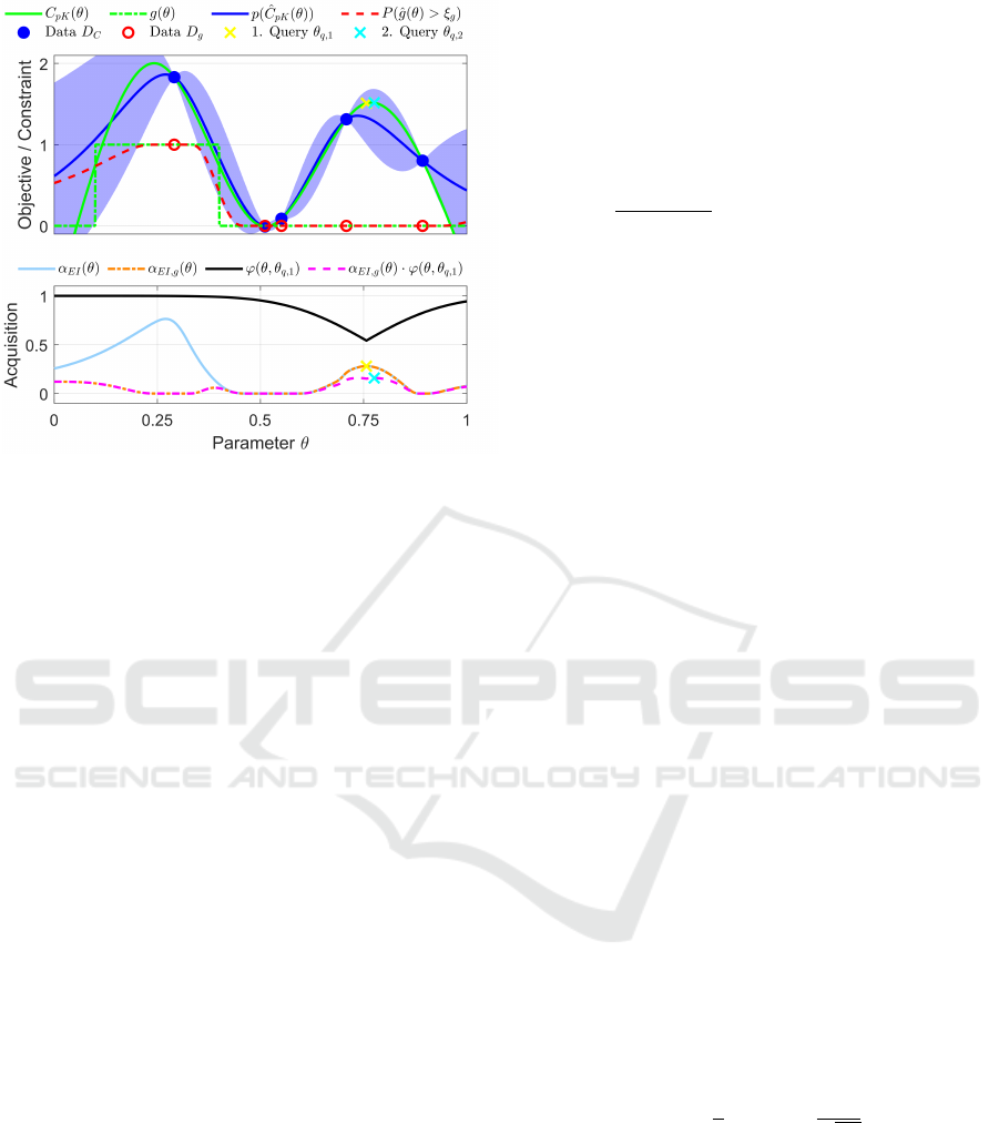
Figure 4: Illustrative representation for an iteration of our

BO method in the one-dimensional case with one control

parameter. A detailed explanation can be found in the text.

to the previous data. These steps are repeated un-

til, e.g., a predetermined number of experiments have

been performed. Then, the best control parameter-set

with respect to (3) is selected from all observations

collected so far.

In the following we present a detailed explana-

tion of the execution of our batch constrained BO

approach. For a better understanding of subsequent

explanations, the reader is referred to Algorithm 1

and Figure 4. Algorithm 1 summarizes the steps of

our BO implementation. In addition, Figure 4 shows

the relationships of the considered functions during

one iteration for a one-dimensional example. Note

that the application to the bonding process is multi-

dimensional. The assumption here is that we already

have 5 evaluations of the real unknown functions.

These are represented by the blue and red circles in

the upper image. In addition, the true function C

(θ)

for the process capability index and the constraint

g(θ) are shown in solid and dashed green lines. With

reference to the objective function, we also see the

current Gaussian process assumption in blue. Here,

the solid line is the mean and the shaded area is the

standard deviation (in comparison to (7) and (10)).

A key component in step 2.) is the so-called acqui-

sition function that deﬁnes the underlying optimiza-

tion problem. The acquisition function is required to

derive the new parameter conﬁguration from the two

sources of information available from the Gaussian

process, i.e. the mean µ

(θ) and the uncertainty in

form of the variance σ

(θ). Here, we consistently use

the criterion of expected improvement

(θ) = E[max(0,

(θ) −ξ

)]

∞

(

(θ) −ξ

)N (µ

(θ),σ

(θ)) d

= σ

(θ)φ(γ(θ)) + (ξ

−µ

(θ))(1 −Φ(γ(θ))),

γ(θ) =

−µ

(θ)

(11)

where φ(·) is the probability density function and Φ(·)

is the cumulative distribution function of a standard

normal distribution. The main idea here is to focus

on the probability measure above a certain threshold

and use the center of this measure as a point to

determine the next query location. The criterion thus

strikes a balance between exploration and exploita-

tion.

In the lower picture of Figure 4 we see the evalu-

ation of the objective Gaussian process from the up-

per picture. The solid light blue line shows the ex-

pected improvement acquisition function from Equa-

tion (11). The associated threshold value ξ

is 1. This

is why the function is close to 0 in a range around the

parameter value of 0.5. Maximizing this function re-

sults in the real functions from the upper image being

evaluated near the left data point. This is the global

maximum, however the constraint is not met in this

region (g(θ) = 1 for θ ∈ (0.1, 0.4)). Thus, an evalua-

tion is not desired at this location.

Next, we turn our consideration to the constraint

for preventing tool collisions. Here the probability

density distribution p( ˆg(θ) | D

) = N (µ

(θ),σ

(θ))

is given. In contrast to the objective function, we are

not interested in the speciﬁc value for the constraint,

but rather in the probability for the occurrence of a

tool collision. For this reason, we integrate over the

probability density function from a certain threshold

P( ˆg(θ) > ξ

) =

∞

N (µ

(θ),σ

(θ))dθ



1 + erf



θ−µ

√

2σ



(12)

where erf(·) is the so called error-function. We treat

g(θ) = 0 as a soft constraint and multiply the acquisi-

tion function (11) by the counter probability of (12),

which yields

EI,g

(θ) = α

(θ)



1 −P( ˆg(θ) > ξ

)



. (13)

In this way, even favorable regions where the proba-

bility for a tool collision is high and the acquisition

function value is also high are still taken into account

ICPRAM 2022 - 11th International Conference on Pattern Recognition Applications and Methods

388

Algorithm 1: Batch Constrained Bayesian Optimization.

1: Input: Initial dataset D

= {θ

,µ

,σ

}, with i = 1,...,n

init

, batchsize n

batch

, iteration budget n

budget

mean functions m

and covariance functions k

, threshold values ξ

,ξ

, lower speciﬁcation

limit LSL.

2: for i = 1 to n

budget

3: Update Gaussian process hyper-parameters w.r.t. µ

,σ

based on D

. ▷ By solving (6)

4: for b = 1 to n

batch

5: Calculate b-th batch element θ

q,b

. ▷ By solving (15)

6: end for

7: Evaluate at θ

q,b

and receive {µ

,q,b

,σ

,q,b

q,b

}, for b = 1,..., n

batch

8: Attach new data to existing one D

i+1

= D

∪ {θ

q,b

,µ

,q,b

,σ

,q,b

q,b

9: end for

10: Returns: θ

,with r = indexmax

r,g

pK,r=1,...,n

init

batch

iter

and can thus be evaluated. This is especially impor-

tant for the early iterations where a small amount of

data is available and the Gaussian process with re-

spect to the constraint provides poor predictions.

The red dashed line in the upper image of Fig-

ure 4 shows the probability of a tool collision (12).

The threshold ξ

was set to 0.5. It can be seen

that the probability of a tool collision on the right

side is broadly zero, whereas the probability changes

smoothly to a value of one for the only observed tool

collision on the left side. For a diminishing value θ

towards zero, the probability drops again as we ex-

trapolate here and have chosen an optimistic mean

function of zero. The orange dashed line in the lower

image shows the weighting of the expected improve-

ment acquisition function with the counter probability

for a tool collision (13). The left area is discounted

down so that the new maximum is assumed to be on

the right and should be evaluated at the location of the

yellow cross.

Up to this point, we have only considered one

experiment in each iteration. With respect to ultra-

sonic wire bonding, the ﬁrst step is to insert a blank

substrate plate into the bonding machine and auto-

matically bond it with the selected control parame-

ters. Then, the substrate plate must be removed from

the bonding machine and placed into the shear tester,

where the shear resistance is measured. The result-

ing values are then manually entered into the database

on which the BO algorithm operates. Since bond-

ing and shearing are relatively fast and automated, it

is reasonable to calculate multiple control parameter-

sets directly in one BO iteration instead of one and to

evaluate them in parallel. These parallel evaluations

are called batches and we will use the approach from

(Gonzalez et al., 2016) for our implementation. To

further motivate the usage of batches, we take a look

at the speciﬁc time needed for one iteration. This time

is composed of the time to calculate the query loca-

tion t

calc

, the time needed to prepare the experiment

prepare

and the time spent for the actual evaluation

eval

. The total time then sums up to T

single

= (t

calc

prepare

eval

)·n

iter

, where n

iter

is the number of itera-

tions. For n

batch

batch elements the total time amounts

to T

batch

= (n

batch

calc

prepare

batch

eval

)·

iter

batch

un-

der the assumption that the preparation time does not

change and the time for calculation and evaluation

scales linearly, which is a rather pessimistic assump-

tion in most cases. For our experimental setting, the

following times can be roughly estimated (in sec-

onds) as t

calc

= 10,t

prepare

= 100,t

eval

= 50. With

iter

= 100 and n

batch

= 6, the total times correspond

to T

single

= 4 hours and T

batch

= 1.9 hours, which is

equivalent to a reduction of more than 50%. However,

this reduction comes at the price of a decreased efﬁ-

ciency because all identiﬁed batch elements are based

upon the same Gaussian processes and therefore, it

is only updated after all batch elements are evaluated

and not one by one.

To accommodate multiple query locations, the

weighted acquisition function must be further modi-

ﬁed. The approach in (Gonzalez et al., 2016) recom-

mends the use of a so-called local penalizer

ϕ(θ,θ

) =

erf



−

2σ

(θ

)



∥G∥

∥θ −θ

∥

−ξ

+ µ

(θ

)





with G =

dµ

(θ)

dθ



θ=θ

(14)

This penalizer depends on the control parameters θ

and on a speciﬁc query location θ

, which is the pre-

viously selected batch element. The strength of the

penalty depends on the norm of the gradient of the

posterior mean function ∥G∥

times the distance be-

Batch Constrained Bayesian Optimization for Ultrasonic Wire Bonding Feed-forward Control Design

389

tween the parameters under consideration and the pre-

vious batch element ∥θ−θ

∥

. Other components are

the posterior mean µ

(θ

) and variance σ

(θ

) eval-

uated at the previous batch element and the threshold

value ξ

. The basic idea is to use a penalizer for each

calculated batch element and determine the next batch

element by the product of the soft constrained acqui-

sition function and all local penalizers

q,b

= argmax

(

EI,g

(θ) if b = 1,

EI,g

(θ)

∏

b−1

i=1

ϕ(θ,θ

q,i

) else,

(15)

for b = 1,...,n

batch

. In summary, the individual opti-

mization problems (15) are solved sequentially one

after the other until all n

batch

batch-elements have

been calculated. Afterwards, all batch elements re-

spectively control parameters are tested on the real

system. Figure 4 illustrates this concept by the black

solid line representing the local penalizer (14) at the

location of the yellow cross. The product of the black

line and the orange dashed line gives the magenta

dashed line, whose maximum value is at the position

of the cyan cross (compare to (15)). For this illus-

trative example the total number of batch elements

is two. Further batch elements can be calculated by

additional local penalizers as required by the applica-

tion.

4 APPLICATION

In order to obtain high quality results for the bond

joints despite the complexity of the process in ultra-

sonic bonding, our proposal is to apply BO for deter-

mining the optimal feed-forward control. For this pur-

pose, in this section we will ﬁrst list our experimental

settings regarding our speciﬁc equipment and chosen

inputs for Algorithm 1 (Subsection 4.1). Then, the re-

sults from the real experiments are described and an-

alyzed to clearly show the beneﬁts in ultrasonic bond-

ing (Subsection 4.2). To further strengthen the results,

we also show the application of our method to a sim-

ulated bonding process, allowing us to study the be-

havior for many more initial conditions (Subsection

4.3).

4.1 Experimental Settings

For our experiments we used a Hesse Mechatronics

automatic wire bonder BJ955 with an RBK03 bond

head. Aluminum dibond plates are used as the sub-

strate. The wire also consists of aluminum, has a

diameter of 500 µm and is manufactured by Tanaka,

type TANW Soft 2. Shear strengths are measured us-

ing a Xyztec Sigma shear tester.

With respect to Algorithm 1, we set the num-

ber of initial experiments n

init

to 10, the number of

batch elements n

batch

to 6, the iteration budget n

budget

to 15, which limits the number of experiments to

init

+ n

batch

budget

= 100, and the threshold values

to 2 and ξ

to 0.5. The lower speciﬁcation limit

LSL is 2500 cN and the number of bonds per control

parameter-set n

rep

is 10. The search space of the con-

trol parameters is box-constrained with lower limit θ

and upper limit θ

(see Table 1).

All Gaussian processes assume the 3/2-Mat

ern

covariance function described in (5). In order to

compare the hyper-parameters we also normalized

the inputs to the unit interval via the lower and up-

per bounds from Table 1. Algorithm 1 was imple-

mented in MATLAB. The optimization of the acquisi-

tion function is solved in two steps via random search

with 1 million candidates. The best candidate is used

as an initial guess for the follow up optimization with

the build-in routine fminsearch

. Note that the mas-

sive number of evaluation of the acquisition function

is unproblematic, since its computational complexity

is low and it can be calculated relatively fast.

4.2 Real-world Results

In this subsection we present the results from the real

bonding process. We compare 4 different approaches

with each other:

• Random Search: A random controller

parametrization is drawn from the uniform

distribution θ

∼ U(θ

,θ

) for every experi-

ment.

• Manual Tuning: A non-expert, who is familiar

with the process and its physical effects, is tun-

ing the control parameters manually. The person

has to choose 6 parametrizations in every itera-

tion, which will then be evaluated in parallel. This

is comparable to the proceeding of Algorithm 1.

All previous experiments can be accessed at any

time in order to draw conclusions for the next

parametrizations.

• BO with a Constant Prior Mean Function: This

is our base case scenario, where no speciﬁc a-

priori knowledge about the process is available.

Therefore, we set the prior mean functions for the

mean shear force and the standard deviation to

constant values, namely m

= 2500 and m

= 60,

More information can be found at math-

works.com/help/matlab/ref/fminsearch.html

ICPRAM 2022 - 11th International Conference on Pattern Recognition Applications and Methods

390

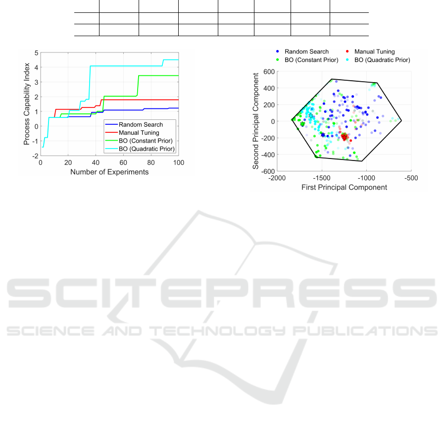
Table 1: Box-constraints for the search space.

[cN] F

[cN]

[V]

[V] T

[ms] T

[ms]

300 375 375 43.3 7.75 5.5 29.5

900 1125 1125 80.6 54.25 38.5 206.5

Figure 5: Progress of the objective over the number of per-

formed experiments. An improvement is only achieved if a

tested control parameterization leads to bonds with a higher

process capability index than any previous parametrization

and the optical criteria are satisﬁed. Otherwise the progress

curve stays constant.

resulting in a rather pessimistic initialization with

a process capability index value of 0.

• BO with a Quadratic Mean Prior Function:

This is a reference scenario, where a quadratic

prior mean function m

(θ) = θ

Aθ + b

θ + c for

the mean shear force is used instead of a constant

one. The mean function for the standard deviation

stays constant. The quantities A, b,c are ﬁtted to

all data gathered from the other three approaches

via least-squares regression.

In Figure 5, we see the progress in the process ca-

pability index over the number of experiments. Con-

stant plateaus indicate that no improvement happened

in the related experiments. Note that a jump in the

objective only occurs if the C

value is higher com-

pared to all previous experiments and the constraint,

with respect to optical criteria, is satisﬁed. All ap-

proaches were given the same 10 initial experiments.

In industrial processes, a minimum C

of 1.33

to 1.67 is typically required (DVS - German Welding

Society, 2017). Random search gets stuck near the

value of 1 pretty fast and no signiﬁcant improvement

happens. From these observations, we suspect that

the surface of the objective function is rather ﬂat for a

large part of the search space. Manual tuning provides

an improvement in efﬁciency. However, after around

50 experiments, no further improvement was found.

On the other hand, BO with a constant prior found a

signiﬁcantly better control, although it was previously

on the same level as manual tuning. We think that the

early random search like behavior is due to initial ex-

Figure 6: Progress in an reduced parameter space. The

transparency indicates the number of the experiment, the

greater the earlier. The stars show the best parameters for

each approach.

ploration of the search space. However, this behav-

ior might be beneﬁcial for later iterations. BO with a

quadratic prior shows the best results and provides the

best control over all approaches. Several experiments

are needed to obtain this parametrization, which in-

dicates that the quadratic prior has some mismatches

to the real objective function. However, the explo-

ration is guided to a region of potentially high qual-

ity parameters, which results in an overall high efﬁ-

ciency. This case shows how a reasonably good, but

not necessarily perfect prior mean function improves

the progress of BO. Instead of a data-driven model,

we might think of a physical model of the process

to improve performance. From a reverse-engineering

perspective, our results show that this physical model

has to imply a quadratic function for the shear force.

We want to investigate this general idea in the future.

Next, we focus on the progress in the param-

eter space, see Figure 6. Since a 7-dimensional vi-

sualization of all parameters would be confusing, we

transformed the data onto a 2-dimensional space by a

principal component analysis (PCA). A singular value

decomposition (SVD) of the data matrix, which is

formed from all parameter values of all experiments,

was calculated. Then, the parameter values were

transformed into a 2-dimensional space via the ﬁrst

two columns of the matrix with the left singular vec-

tors, which are thus assigned to the two largest singu-

lar values. The parameters related to random search

are broadly diversiﬁed as expected. The concentra-

tion of red dots in one area is noticeable. This region

was locally explored by the manual tuner, since the re-

Batch Constrained Bayesian Optimization for Ultrasonic Wire Bonding Feed-forward Control Design

391

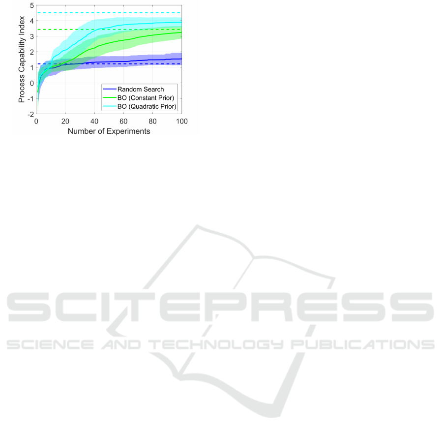
Figure 7: Progress of the objective function value over the

number of experiments in the simulated environment. The

solid lines show the average progress over multiple runs and

the transparent areas indicate two standard deviations. The

dashed lines show the maximum values found for the real

process (compare to Figure 5).

sulting objective function values were relatively good

and the constraint was fulﬁlled. We would classify

the proceeding as safe exploration, where the region

of tested parameters is iteratively expanded. We also

noticed that the overview of the previous experiments

was lost at around 30 to 40 experiments, which is the

explanation for the lack of progress on the objective

function in Figure 5. On the other hand, BO espe-

cially explores the bounds of the search space and fo-

cuses relatively fast on the region where the highest

values were found. For reasons of conﬁdentiality, we

are not permitted to provide the optimal parameters.

4.3 Simulated Results

Since experiments on the real system are time and

cost consuming, we could not investigate the inﬂu-

ence of the initial experiments and therefore the ro-

bustness of each approach. Based on this reason,

we set up Gaussian processes, which are built upon

all data gathered so far, to replace the real system.

Hence, their predictions are relatively accurate. This

virtual environment enables us to test the approaches

used in Subsection 4.2, excluding manual tuning, for

different initial experiments.

Figure 7 shows the dedicated results for 50 differ-

ent runs. First of all, we see that the runs with re-

spect to the real system are reasonable, because they

ﬁt the simulated runs. Furthermore, the used BO

methods outperform random search robustly and con-

verge to high objective function values. The fact that

the global maximum from the measurements (dashed

cyan line) is not reached by quadratic prior BO may

be related to the regularization of the reference Gaus-

sian processes. However, the optimal parameters

found are identical. These results strengthen our hy-

pothesis that BO is appropriate for the control design

of the bonding process.

Another advantageous property of training Gaus-

sian processes with all data is the ability to investi-

gate the learned hyper-parameters η

∗

. Especially the

learned scales reveal the relevance of a given param-

eter dimension to the output. This is called automatic

relevance determination in the literature (Rasmussen

and Williams, 2006).

The hyper-parameters are shown in Table 2. Note

that a direct comparison is possible, since we stan-

dardized the parameter dimensions to the unit inter-

val. The higher the value of the scale l, the smaller

the inﬂuence of the underlying parameter. Regarding

the mean shear force ˆµ

(θ) and the label ˆg, we see

that the normal force of the pre-deformation phase

is less relevant compared to the standard devia-

tion

(θ), which seems plausible, because a sufﬁ-

cient initial contact area is formed by a wide range

of values. On the other hand, the values of the ultra-

sonic voltages (

) have a relatively high impact

on the mean shear force. This also holds for the stan-

dard deviation of the shear force

(θ). However, we

see that the force F

and time T

of the second phase

have the most inﬂuence, which means that these val-

ues have to be chosen with high accuracy for receiv-

ing a low standard deviation. The values for the signal

and noise variance (σ

, σ

) match with the observa-

tions during the experiments.

5 CONCLUSION AND OUTLOOK

Real-world and simulated results showed that the ap-

plication of BO to the feed-forward control design

of ultrasonic wire bonding is very appropriate. The

suggested approach outperforms random search and

manual tuning in terms of efﬁciency and robustness.

We also showed that the incorporation of a quadratic

prior mean function is advantageous and increases the

performance. We see this result as a guideline for fur-

ther research, where we exchange the quadratic prior

with a physical simulation model of the bonding pro-

cess. Our work lays the foundation for this since

it builds upon numerous measurements with a wide

range of control inputs applied to the real bonding

process and is thus well validated. Furthermore, we

investigated the hyper-parameters and discovered that

the touchdown force, which is applied during the pre-

deformation phase, has little inﬂuence on the bond

quality. The mean shear force is sensitive to the volt-

age amplitude values, whereas the variance responds

the most to the normal force in the second phase and

its duration.

ICPRAM 2022 - 11th International Conference on Pattern Recognition Applications and Methods

392

Table 2: Hyper-parameters for the reference Gaussian processes.

GP σ

ˆµ

(θ) 4.4 ·10

13.7 2 1.9 1.7 1.4 2.9 2.6 1.6 ·10

(θ) 1.7 ·10

1.3 1.9 0.2 0.9 0.9 2.3 0.8 335

ˆg 0.3 3 0.7 1.1 0.5 0.5 1 1.3 0.05

Besides a physics-based prior mean function, we

want to investigate other materials, like copper, or dif-

ferent wire diameters. The modiﬁcation of other gen-

eral conditions could also be considered. Our pro-

posed method can be applied in the same way. How-

ever, we can build on the results from this paper and

examine the ﬁeld of transfer learning. A good start-

ing point might be the Gaussian processes which were

trained with all the data points from our experiments.

ACKNOWLEDGEMENTS

The research was funded by the Ministry of Eco-

nomic Affairs, Innovation, Digitalisation and Energy

(MWIDE) of the State of North Rhine-Westphalia

within the Leading-Edge Cluster Intelligent Techni-

cal Systems OstWestfalenLippe (it’s OWL) and by

the Federal Ministry of Education and Research of

Germany (BMBF) within the junior research group

DART of the University of Paderborn. The responsi-

bility for the content of this publication lies with the

authors.

The authors would like to thank Yuqi Liu, Jan Her-

bermann and Fabian Reiling for their assistance dur-

ing the experiments.

REFERENCES

Calandra, R., Seyfarth, A., Peters, J., and Deisenroth, M. P.

(2016). Bayesian Optimization for Learning Gaits un-

der Uncertainty. Annals in Mathematics and Artiﬁcial

Intelligence, 76:5–23.

ıaz-Franc

es, E. and Rubio, F. J. (2013). On the Existence

of a Normal Approximation to the Distribution of the

Ratio of two Independent Normal Random Variables.

Statistical Papers, 54(2):309–323.

DVS - German Welding Society (2017). Test Procedures for

Wire Bonded Joints (Technical Bulletin DVS 2811).

Geißler, U. (2009). Verbindungsbildung und

Gef

ugeentwicklung beim Ultraschall-Wedge-Wedge-

Bonden von AlSi1-Draht. Technische Universit

Berlin, Fakult

at IV - Elektrotechnik und Informatik.

Gogh, B., Benner, T., Seppaenen, H., Tszeng, C., and

Sepehrband, P. (2020). An Oxide Wear Model of Ul-

trasonic Bonding. International Symposium on Micro-

electronics, 2020:222–229.

Gonzalez, J., Dai, Z., Hennig, P., and Lawrence, N. (2016).

Batch Bayesian Optimization via Local Penalization.

In AISTATS 2016; 19th International Conference on

Artiﬁcial Intelligence and Statistics.

Harman, G. (2010). Wire Bonding in Microelectronics.

McGraw-Hill.

Hunstig, M., Schaermann, W., Broekelmann, M.,

Holtkaemper, S., Siepe, D., and Hesse, H. J.

(2020). Smart Ultrasonic Welding in Power Elec-

tronics Packaging. In CIPS 2020; 11th International

Conference on Integrated Power Electronics Systems,

pages 1–6.

Jones, D. R., Schonlau, M., and Welch, W. J. (1998).

Efﬁcient Global Optimization of Expensive Black-

Box Functions. Journal of Global Optimization,

13(4):455–492.

Kelly, M. (2017). An Introduction to Trajectory Optimiza-

tion: How to Do Your Own Direct Collocation. SIAM

Review, 59(4):849–904.

Long, Y., Twiefel, J., and Wallaschek, J. (2017). A Re-

view on the Mechanisms of Ultrasonic Wedge-Wedge

Bonding. Journal of Materials Processing Technol-

ogy, 245:241–258.

Mayer, M. and Schwizer, J. (2002). Ultrasonic Bond-

ing: Understanding How Process Parameters Deter-

mine the Strength of Au-Al Bonds. Symposium on

Microelectronics, IMAPS, Denver.

Neumann-Brosig, M., Marco, A., Schwarzmann, D., and

Trimpe, J. S. (2020). Data-efﬁcient Auto-tuning with

Bayesian Optimization: An Industrial Control Study.

IEEE Transactions on Control Systems Technology,

28(5):730–740.

Rasmussen, C. E. and Williams, C. (2006). Gaussian Pro-

cesses for Machine Learning. MIT Press.

Schemmel, R., Krieger, V., Hemsel, T., and Sextro, W.

(2020). Co-Simulation of MATLAB and ANSYS for

Ultrasonic Wire Bonding Process Optimization. In

2020 21st International Conference on Thermal, Me-

chanical and Multi-Physics Simulation and Experi-

ments in Microelectronics and Microsystems.

Shahriari, B., Swersky, K., Wang, Z., Adams, R. P., and

de Freitas, N. (2016). Taking the Human Out of the

Loop: A Review of Bayesian Optimization. Proceed-

ings of the IEEE, 104(1):148–175.

Snoek, J., Larochelle, H., and Adams, R. P. (2012). Prac-

tical Bayesian Optimization of Machine Learning Al-

gorithms. In Pereira, F., Burges, C. J. C., Bottou, L.,

and Weinberger, K. Q., editors, Advances in Neural

Information Processing Systems, volume 25. Curran

Associates, Inc.

Unger, A., Hunstig, M., Meyer, T., Br

okelmann, M., and

Sextro, W. (2018). Intelligent Production of Wire

Bonds using Multi-Objective Optimization – Insights,

Batch Constrained Bayesian Optimization for Ultrasonic Wire Bonding Feed-forward Control Design

393

Opportunities and Challenges. International Sympo-

sium on Microelectronics, 2018(1):572–577.

Unger, A., Sextro, W., Althoff, S., Meyer, T., Br

okelmann,

M., Neumann, K., Reimann, R. F., Guth, K., and

Bolowski, D. (2014). Data-driven Modeling of the

Ultrasonic Softening Effect for Robust Copper Wire

Bonding. In Proceedings of 8th International Confer-

ence on Integrated Power Electronic Systems, volume

141, page 175–180.

ICPRAM 2022 - 11th International Conference on Pattern Recognition Applications and Methods

394