Constrained CP-nets Similarity
Hassan Alkhiri and Malek Mouhoub
a
University of Regina, 3737 Wascana Parkway, Regina, Canada
Keywords:
Qualitative Preferences, CP-net, Constraint Solving.
Abstract:
The Conditional Preference Network (CP-net) is one of the widely used graphical models for representing and
reasoning with qualitative preferences under ceteris paribus (“all else being equal”) assumptions. CP-nets
have been extended to Constrained CP-nets (CCP-nets) in order to consider constraints between attributes.
Adding constraints will restrict agent preferences, as some of the outcomes become infeasible. Aggregating
CCP-nets (representing different agents) can be very relevant for multi-agent and recommender systems. We
address this task by defining the notion of similarity between CCP-nets. The similarity is computed using
the Hamming distance (between the outcomes of the related pair of CCP-nets) and the number of preference
statements shared by both CCP-nets. We propose an algorithm to compute the distance between a pair of CCP-
nets, based on the similarity we defined. In order to evaluate the time performance of our proposed algorithm,
we conduct several experiments and report the related results.
1 INTRODUCTION
Over the years, various preference models have been
proposed, including mathematical models like val-
ued constraint satisfaction problems and C-semirings,
logic-based models like an answer set optimization,
and graphical models with conditional preference net-
works. Preferences are considered to be critical, and
they would express the agent’s desire in a declara-
tive manner (Domshlak et al., 2011; Racharak et al.,
2016; Moussa, 2019; Goldsmith and Junker, 2008).
The choice of an agent is known to be driven ratio-
nally by the underlying preference model (Loreggia
et al., 2018a). Thus, it is crucial to infer the models
that would reflect the user’s preference, responsible
for the decision and action recommendations (Lang,
2010; Rossi et al., 2004; Ricci et al., 2011; Racharak
et al., 2016).
Preference elicitation, representation, and reason-
ing play a significant role in the area of decision-
making (Bonnefon et al., 2016; Boutilier et al., 2004a;
Alanazi et al., 2020). However, preferences often
come with a set of requirements, including those from
the agents . Both preferences and constraints act on
the agent’s desires to get a set of Pareto optimal out-
comes (Alanazi and Mouhoub, 2016). Managing con-
straints and preferences is critical for most real-world
applications. For instance, one of the crucial aspects
a
https://orcid.org/0000-0001-7381-1064
of a successful system is to take into account user’s re-
quirements and desires to make decisions efficiently
and correctly (Mohammed et al., 2015). These in-
clude taking the best outcome feasibility under con-
sideration (Boutilier et al., 2004b; Balke and Wagner,
2003). Furthermore, qualitative approaches (Balke
and Wagner, 2003) have been adopted to describe user
preferences. These models allow agents to express
their preference by comparison, such as: “I prefer
Beef to Fish”. Conditional preferences might be con-
sidered, such as: “if the main dish includes Beef, I pre-
fer fries to rice as a side dish”. A Conditional Pref-
erence Network (CP-net) (Boutilier et al., 2004a) is
a graphical model used to represent conditional pref-
erences under ceteris paribus (“all thing else being
equal”) semantics, in a compact form. Comparing
CP-nets related to multiple agents’ preferences and
aggregating them has attracted the attention of many
researchers in Artificial Intelligence, including multi-
agent systems, and recommender systems (Balke and
Wagner, 2003; Loreggia et al., 2018b; Yager, 2001;
Dalla Pozza et al., 2011). More precisely, there is a
need to utilize different agents’ preferences over a set
of possibly associated attributes(Moussa, 2019). The
goal here can be to extract common decision patterns
and recommendations from a group of customers
based on their preferences. Moreover, we might need
to compare the preferences of two agents or those
between a group of agents and a particular one. In
226
Alkhiri, H. and Mouhoub, M.
Constrained CP-nets Similarity.
DOI: 10.5220/0010802900003116
In Proceedings of the 14th International Conference on Agents and Artificial Intelligence (ICAART 2022) - Volume 3, pages 226-233
ISBN: 978-989-758-547-0; ISSN: 2184-433X
Copyright
c
 2022 by SCITEPRESS – Science and Technology Publications, Lda. All rights reserved

this regard, the authors in (Loreggia et al., 2018b) de-
fine the notion of distance between CP-nets, by gen-
eralizing the Kendall-Tau distance between partial or-
ders. In contrast, in (Wang et al., 2017) an approach
is proposed to capture the similarity agreement be-
tween users, based on their preferences. The latter are
represented with CP-nets. Preference comparison can
be addressed by either measuring the distance of dis-
agreement or the similarity agreement between agents
preferences. A similar work has been conducted on
Lexicographic Preference trees (Li and Kazimipour,
2018). In the latter work, the aim is to calculate the
dissimilarity and distance between agents, each rep-
resented by an LP-tree. In (Racharak et al., 2016),
the authors propose a new similarity measure for the
Description Logic, to present the notion of a general
preference profile.
In this paper, we investigate on these types of sim-
ilarities, when constraints are involved. This can be
very relevant in many real world scenarios, given that
users’ desires often come with a set of requirements.
In this regard, our intent is to define the similarity be-
tween constrained CP-nets (CCP-nets). To achieve
this goal, we redefine the notion of distance (between
CP-nets) in order to consider constraints. In addi-
tion to adopting the Hamming distance between CCP-
nets, we also rely on the number of worsening flips as
a measure of the distance between outcomes. Here,
we assume that the CCP-nets we are considering are
acyclic, and share the same constraints and depen-
dency graph (the underlying CP-nets are isomorphic).
The Hamming distance between a pair of CCP-nets is
computed based on the Conditional Preference Table
(CPT) difference. A CPT is a set of statements rep-
resenting conditional preferences in a compact form.
The total number of CPTs statements corresponds
to the size of the corresponding CCP-net. In other
words, the CCP-net size is defined as the sum of all
attributes CPT statements. Each order of a pair of out-
comes is deduced by a given CPT statement. Measur-
ing the similarity between two CCP-nets consists of
checking their respective consistency and comparing
their respective outcome orders. Comparing the order
of outcomes in two CCP-nets corresponds to compar-
ing their respective CPT statements.
In this regard, we propose an algorithm to measure
the distance between CCP-net structures, based on the
similarity we defined. The main objective here is to
compare two CCP-nets according to their feasibility
of outcomes, while minimizing the disagreement be-
tween their respective preferences. The time perfor-
mance of our algorithm has been assessed by the ex-
periments we conducted and reported in this paper.
2 BACKGROUND
Preferences and constraints are ubiquitous and usu-
ally occur together in many real world applications.
In this regard, both will be considered as part of the
agent’s decision making. For example, if an agent
wants to order a meal, she may unconditionally prefer
certain dishes or drinks over others. Some preferences
can be conditional, such as preferring fries over rice
for a side dish, if the main dish is Beef. The agent may
also have a budget that restricts the possible meals she
can take.
In this paper we adopt the CCP-net framework for
managing both preferences and constraints. In the fol-
lowing, we will first present the CP-net mode, fol-
lowed by the CCP-net.
2.1 CP-net
A CP-net (Boutilier et al., 2004a) is a graphical model
that is used to represent and reason with conditional
qualitative preference under the semantics of ceteris
paribus (“all else being equal”). The CP-net allows
to express complex conditional preferences in a com-
pact and natural representation. The CP-net is repre-
sented as a Directed Dependency Graph (DDG) to-
gether with Conditional Preference Tables (CPT s).
The DDG includes a set of nodes (attributes) X =
{X
1
,... ,X
n
}, where each is associated with a finite
domain of possible values, D(X
i
). A child node in
the DDG is connected by a dependency arc to a set of
parent nodes P(X
i
). Furthermore, a CPT (X
i
) is asso-
ciated to each node X
i
to denote a set of ceteris paribus
preference statements. These statements allow us to
express preference orderings over the attribute values
of X
i
, given the values assigned to P(X
i
). The relation
 denotes the preference relation among attributes
values. For example, the conditional preference rela-
tion a
1
: b
1
 b
2
expresses the fact that attribute value
b
1
is preferred to value b
2
for attribute X2 if its parent
node X
1
has been assigned value a
1
.
A CP-net is illustrated in Figure 1. This CP-net
corresponds to the following scenario.
Example 1
Anila plans to order a meal from a restaurant.
She then faces numeral choices such as A:
Main Dishes (i.e., a
1
:Beef or a
2
:Chicken), B:
Side Dishes (i.e., b
1
:Salad or b
2
:Fries), and
C: Drink (i.e., c
1
: Red Wine or c
2
: White
Wine). As shown in Figure 1, Anila has an
unconditional preference for Main and Side
Constrained CP-nets Similarity
227

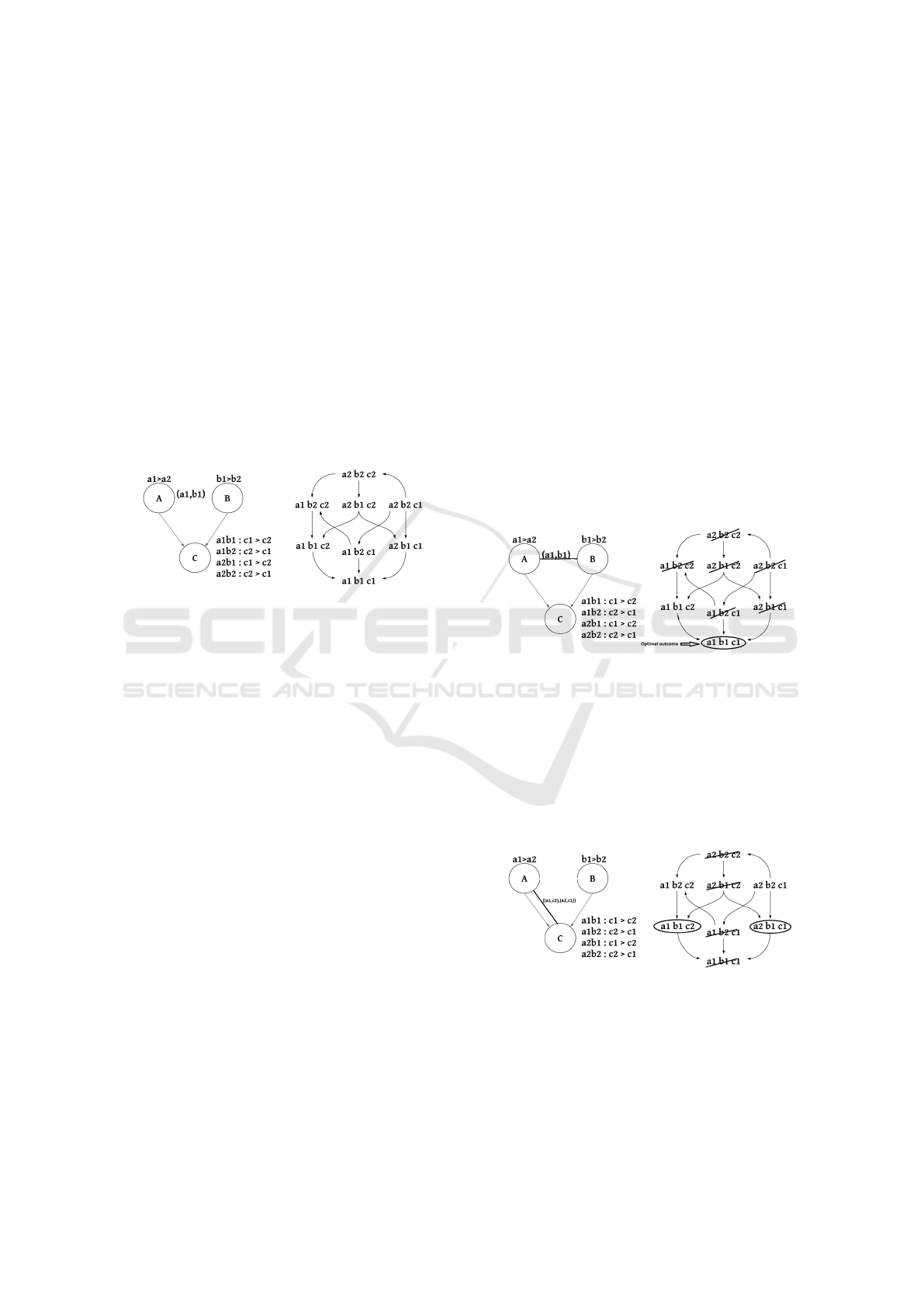
dishes. According to the CPT s, Anila un-
conditionally prefers to have Beef rather than
Chicken as Main dishes and Salad to Fries as
Side dishes. Anila has a conditional prefer-
ence on Drink depending on Main and Side
dishes, respectively, depending on what she
gets for Main and Side Dishes. If she takes
Beef and Salad, she will prefer to have Red
wine for Drink. At the same time, she wants to
have White wine if the Main and side dishes
are chicken and fries, respectively.
A CP-net has one optimal outcome that can be ob-
tained using a sweep forward procedure. This pro-
cedure traverses the CP-net graph following a topo-
logical order and assigns each variable’s best value
accordingly until a complete outcome is obtained
(Boutilier et al., 2004a).
Figure 1: A CP-net (left) and its induced graph (right).
The semantics of CP-nets follows the idea of
worsening flip. One outcome, o
1
, is better than (dom-
inates) another outcome, o
2
if a chain of worsen-
ing flips from o
1
to o
2
(Lang, 2010). A worsening
flip is a variable value changing to a less preferred
value according to the CPT for that variable. For in-
stance, in Figure 1, let us consider o
1
= (a
1
b
1
c
1
) and
o
2
= (a
1
b
1
c
2
). Then, going from o
1
to o
2
is a wors-
ening flip, obtained by flipping value c
1
of variable C
to c
2
. Similarly, going from o
2
to o
1
is an improv-
ing flip, obtained by flipping value c
2
of variable C to
c
1
. Consequently, o
1
= (a
1
b
1
c
1
) dominates (a
1
b
1
c
2
).
The right chart of Figure 1 shows the preference graph
over all the outcomes induced by the CP-net. In the
induced graph, an arc from outcome o
i
to outcome o
j
corresponds to an improving flip and indicates that o j
is preferred to (dominates) oi, according to the CP-
net.
2.2 Constrained CP-net (CCP-net)
The Constrained CP-net (CCP-net) model (Boutilier
et al., 2004b; Alanazi and Mouhoub, 2016) is an ex-
tension of the CP-net to a set of constraints. More for-
mally, a constrained CP-net is a pair (N,C), where N
is a CP-net and C is a set of constraints restricting the
values that the CP-net variables can take. Adding con-
straints may reduce the set of possible outcomes. The
left chart of Figure 1 is a CP-net that will be extended
to a CCP-net if we add the constraint, C = c(A,B)
(listing the eligible tuple, (a
1
,b
1
)), as shown by edge
connecting node A to node B. In general, the con-
straint graph (reduced to nodes A and B, with the edge
between them, in our example) is called a constraint
network and is often formalized as a Constraint Sat-
isfaction Problem (CSP). A CSP is a tuple (X,C,D)
where X is a set of variables, each defined on a do-
main in D
i
∈ D, and C is a set of constraints restring
the values that the variables can simultaneously take.
The idea of a CCP-net (N,C) is to add to the CP-
statements of the CP-net, a set of constraints such that
some outcomes are feasible and not dominated by any
other outcome. These outcomes form the Pareto op-
timal set (Boutilier et al., 2004b). According to our
CCP-net in Figure 1, we only have two feasible out-
comes: {(a
1
b
1
c
2
),(a
1
b
1
c
1
)}, with (a
1
b
1
c
1
) being the
optimal outcome. This change is illustrated in Figure
2.
Figure 2: A Constrained CP-net (CCP-net) and (left) and its
induced graph (right).
In case we change the constraint to C = {c(A,C) =
{(a
1
,c
2
),(a2,c
1
)}} as shown in Figure 3 then our op-
timal outcome is no longer feasible. In this particu-
lar situation, we have two Pareto optimal outcomes:
(a
1
b
1
c
2
) and (a2b
1
c
1
) (these are the next two best so-
lutions, after (a
1
b
1
c
1
), as we can see on the induced
graph of Figure 3).
Figure 3: A Constrained CP-net (CCP-net) and (left) and its
induced graph (right).
ICAART 2022 - 14th International Conference on Agents and Artificial Intelligence
228

3 CONSTRAINED CP-NETS
SIMILARITY
In what follows, we will assume that all CCP-nets are
acyclic and binary (each attribute domain contains ex-
actly two values). Let us consider two constrained
CP-nets CCP
1
= (N
1
,c
1
) and CCP
2
= (N
2
,c
2
) repre-
senting constraints and preferences of two agents. To
compute the similarity between two CCP-nets, CCP
1
and CCP
2
, the following conditions should be satis-
fied.
1. CCP
1
and CCP
2
have the same set of variables,
V = X
1
,. .. ,X
n
, where each variable X
i
is defined
on the same domains of values, D(X
i
).
2. The underlying graphs for N
1
and N
2
are isomor-
phic (same dependency graph structure).
3. c
1
= c
2
: both CCP
1
and CCP
2
share the same un-
derlying constraint graph.
In the above, let Pa(X
i
) be the set of parent’s attributes
which X
i
depends on, and let O be the set of outcomes
for both CCP
1
and CCP
2
.
The similarity between CCP
1
and CCP
2
can be ex-
pressed using the Hamming distance. Let us first de-
fine the Hamming distance between outcomes.
Definition 1. The Hamming distance between a pair
of outcomes, HD(o,o
0
) (o, o
0
∈ O), is the number of
variables in the outcomes for which the values differ.
More formally, the Hamming distance can be
computed as follows.
HD(o,o
0
) = |{X
i
∈ V : o[X
i
] 6= o
0
[X
i
]}| (1)
In the above, o[X
i
] (respectively o
0
[X
i
]) denotes the
value assigned to variable X
i
in o (respectively in o
0
).
In the example of Figure 1, HD(a
1
b
1
c
2
,a2b
1
c
1
) = 2,
given that both outcomes differ in the values of vari-
ables A and C. Note that HD(o,o
0
) = HD(o
0
,o) for
all (o,o
0
) ∈ O and that HD(o,o
0
) = 0 if and only if
o = o
0
. Finally, 0 ≤ HD(o,o
0
) ≤ n, where n = |V |.
If our focus is on the optimal outcomes, then we
can define the similarity by the Hamming distance
between the best outcomes of both CCP-nets. This
however, requires us to solve both CCP-nets and then
apply the Hamming distance between the best out-
comes. Solving the CCP-net is NP-hard and requires
an algorithm of exponential time cost (Boutilier et al.,
2004b; Alanazi and Mouhoub, 2016). In case we have
a set of Pareto optimal solutions when solving one
or both CCP-nets then we need to compute the Ham-
ming distance between each possible pair. We will
then compute the sum (TotalHD) of each resulting
Hamming distance (of each pair) and divide the re-
sult by the total number of possible pairs. We call
disHCCP this distance that is defined as follows.
TotalHD =
∑
o∈S(CCP
1
)∧o
0
∈S(CCP
1
)
HD(o,o
0
) (2)
disHCCP(CCP
1
,CCP
2
) =
TotalHD
|S(CCP
1
)| × |S(CCP
2
)|
(3)
S(CCP
1
) and S(CCP
2
) are the sets of Pareto opti-
mal solutions for CCP
1
and CCP
2
, respectively.
If, however, we want to measure the similarity be-
tween both CCP-nets then we need to define a dis-
tance capturing the differences between the related in-
duced graphs. More precisely, we can add a penalty
equal to one for every pair of outcomes that differ in
their ordering in CCP
1
and CCP
2
. This will lead to
computing the following distance, disCCP between
CCP
1
and CCP
2
. disCCP(N
1
,N
2
), the similarity (dis-
tance) between the underlying CP-nets, N
1
and N
2
(of
CCP
1
and CCP
2
, respectively) can be defined as fol-
lows.
1. disCCP(N
1
,N
2
) = 1, if the related induced graphs
are identical (all the outcomes in both CCP-nets
are ordered in the same way).
2. disCCP(N
1
,N
2
) = 0, if the related induced graphs
have all the arcs reversed (for each arc in CCP
1
,
the corresponding arc in CCP
2
is in the opposite
direction).
3. 0 < disCCP(N
1
,N
2
) < 1, if the related induced
graphs has some arcs in order and others reversed.
We now define the distance disCCP(CCP
1
,CCP
2
),
in the general case. disCCP(CCP
1
,CCP
2
) quantifies
the similarity between the related induced graphs, as
explained earlier. For that, we first compute the num-
ber of orders (between pairs of outcomes) that are
identical in both induced graphs. We then divide this
number by the number of possible orders in both in-
duced graphs. The resulting ratio will correspond to
disCCP(CCP
1
,CCP
2
). The number of possible orders
is the number of arcs in an induced graph. This num-
ber corresponds to the total number of swaps (wors-
ening or improving flips) and is computed as follows.
tSwap = n × 2
(n−1)
The above can be explained by the fact that swaps
correspond to worsening or improving flips. In either
case, this operation consists of going from one out-
come to another by flipping one variable value. Given
a CCP-net with n variables, we have 2
n−1
possibilities
for each of the n swapped variables.
In order to compute the number of identical or-
ders (arcs or swaps) for the induced graphs in two
CCP-nets, CCP
1
and CCP
2
, we can first identify the
CPT statements (in each CPT) that are identical in
Constrained CP-nets Similarity
229

both CCP-nets. Then, for each identical CPT state-
ment, we compute the number of identical swaps that
it induces. The total number of these swaps, for all
identical CPT statements, will be the total number of
identical swaps in both CPTs.
For a given variable X
i
, the number of swaps a
given CPT preference statement induces is equal to:
2
(n−|Pa(X
i
)|−1)
. This number is justified by the fact
that there are n − |Pa(X
i
)| − 1 possibilities for a given
swap, induced by its related CPT statement. The total
number of identical swaps is as follows.
dSwap =
∑
X
i
∈X
nbIdStatements(X
i
) × 2
(n−|Pa(X
i
)|−1)
In the above equation, nbIdStatements(X
i
) is the
number of X
i
’s CPT statements that are identical in
both CPT-nets. Finally, disCCP(CCP
1
,CCP
2
) can be
computed as follows.
disCCP(CCP
1
,CCP
2
) =
dSwap
tSwap
(4)
In order to compute disCCP(CCP
1
,CCP
2
), we de-
signed a procedure that traverses both CCP
1
and CCP
2
in a topological order and checks that the three condi-
tions we listed for similarity are met. While doing so,
the algorithm identifies those CPTs that are identical
in both CCP-nets and computes disCCP(CCP
1
,CCP
2
)
accordingly.
Algorithm 1 lists the pseudo-code of our proce-
dure.
Algorithm 1: disCCP(CCP
1
,CCP
2
).
Input: CCP
1
= (N
1
,c
1
) and CCP
2
= (N
2
,c
2
)
Output: disCCP(CCP
1
,CCP
2
)
1 X = {X
1
,... , X
n
} is the set of variables in CCP
1
2 Y = {Y 1,. . .,Y
n
} is the set of variables in CCP
2
3 CX
i
∈ c
1
(respectively CY
i
∈ c
2
): set of constraints
including X
i
(respectively Y
i
) it their scope
4 nbIdenticalS = 0
5 dSwap = 0
6 tSwap = n × 2
n−1
7 if X = Y then
8 n = |X |
9 Order the variables in X and Y, in topological
order
10 for X
i
∈ X ∧ Y
i
∈ Y do
11 if (D(X
i
) = D(Yi)) ∧ (CX
i
=
CY
i
) ∧ (Pa(X
i
) = Pa(Y
i
)) then
12 nbIdenticalS = |CPT(N
1
,X
i
) ∩
CPT(N
2
,Y
i
) |
13 dSwap += nbIdenticalS× 2
n-|Pa(X)|-1
14 Return
dSwap
tSwap
Example 2
Suppose we have the CCP-net in Figure 4,
representing the preferences for another per-
son, Alice. According to Figures 1 and 4, both
Anila and Alice have the same preferences for
Attributes A and B (respectively representing
the main and side dish). In addition, their
preferences for C (drink) are dependent on
both the main and side dishes. They also both
share the same constraint. However, 2 out of
4 preference statements are different. The first
and second statements are different, as we can
see in both figures. As a result, 2 arcs are dif-
ferent in the related induced graphs (these 2
arcs are marked in Figure 4).
Figure 4: The CCP-net of another agent.
In this particular case, the similarity between both
CCP-nets will be computed as follows, using equation
4.
disCCP(CCP
1
,CCP
2
) =
dSwap
tSwap
=
2×2
(3−2−1)
3×2
(3−1)
=
2
12
= 0.167
4 EXPERIMENTATION
To assess the time performance of the algorithm com-
puting disCCP, we conducted several experiments on
CCP-nets instances randomly generated using a vari-
ant of the RB model (Xu and Li, 2000). More pre-
cisely, CCP-nets instances are generated using four
input parameters: n, p, α and r. n is the number of
variables, p (0 < p < 1) determines the constraint
tightness (number of incompatible tuples over the
Cartesian product of the constraint’s variables), and
r and α (0 < r, α < 1) are two positive constants. Ac-
cording to (Xu and Li, 2000), the phase transition P
t
is calculated as follows: P
t
= 1 − e
−α/r
. Satisfiable
instances are therefore generated with tightness p<P
t
.
The generation of the underlying CSP (constraint net-
work) of the CCP-net instance will be conducted ac-
cording to the following steps.
1. Select t = r × n × ln (n) random constraints (cor-
responding to pairs of variables).
ICAART 2022 - 14th International Conference on Agents and Artificial Intelligence
230

 sH 



 s 
 s 












z
0





i
 
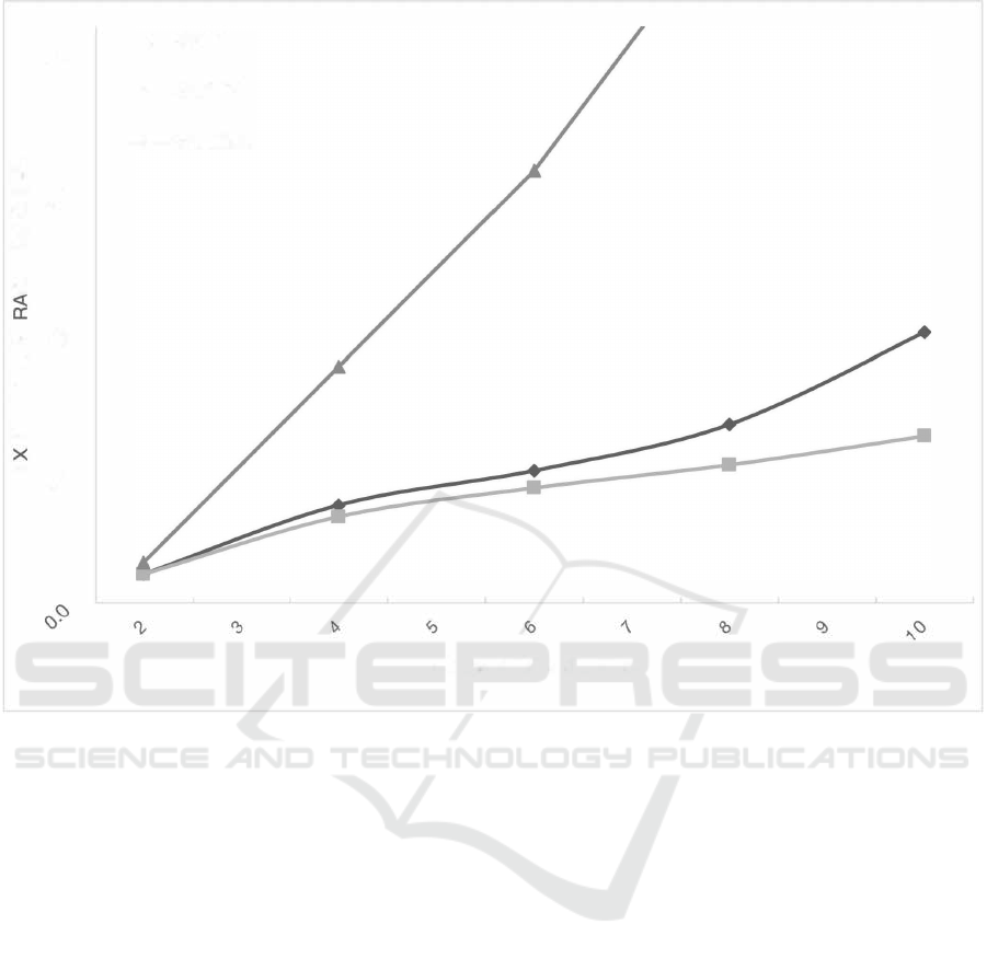
Figure 5: Time needed to compute distance metrics with various numbers of variables.
2. For each constraint, we uniformly select q=p×d
2
incompatible pairs of values, where d = n
α
is the
domain size of each variable. All the variables
will be assigned the same domain corresponding
to the first d natural numbers (0, . . . , d−1).
3. For each constraint, selected incompatible pairs of
values will receive a weight of 0, while each com-
patible pair will randomly receive a weight from
1 to K, where K is provided at input.
The underlying CP-net instance of the CCP-net,
will then be randomly generated as follows.
• Dependencies: For each variable X
i
, we ran-
domly pick up to np parents from {X
0
,. . . , X
i−1
}.
np (0 < np < n), the maximum number of parents,
is provided at input. Note that we always follow
the same order of variables in order to prevent cy-
cles.
• CPT Tables (for each variable X
i
): For each
combination of parents’ values (there are d
np
pos-
sible combinations), randomly generate an order
for all the values of X
i
(there are d! possible or-
ders).
The experiments have been conducted on a Ma-
cOS Catalina version 10.15.2 with 16 GB RAM and
2.6 GHz Intel Core i7.
In the first set of experiments, we eval-
uate three approaches computing the distance:
disHCCP,disCCP and dicExhau. The latter is a base-
line exhaustive method that consists of computing
the distance between each possible outcome pairs for
both CCP-nets.
Figure 5 reports the average running time (in mil-
liseconds) spent by each approach versus the number
of attributes (varying from 2 to 10). The tightness
value is set to 0.4.
The results clearly show the two methods per-
form better than the exhaustive approach. Moreover,
as the number of attributes increases, the exhaustive
approach takes much longer time. For instance, for
10 variables, the exhaustive approach takes approxi-
mately 5000 ms while only 50 and 20 ms are required
by dicCCP.
In the second set of experiments, we vary the con-
straint tightness p from 0.1 to 0.6. The number of
variables is fixed to 50. The results presented in Fig-
ure 6 show again that the exhaustive approach is the
Constrained CP-nets Similarity
231

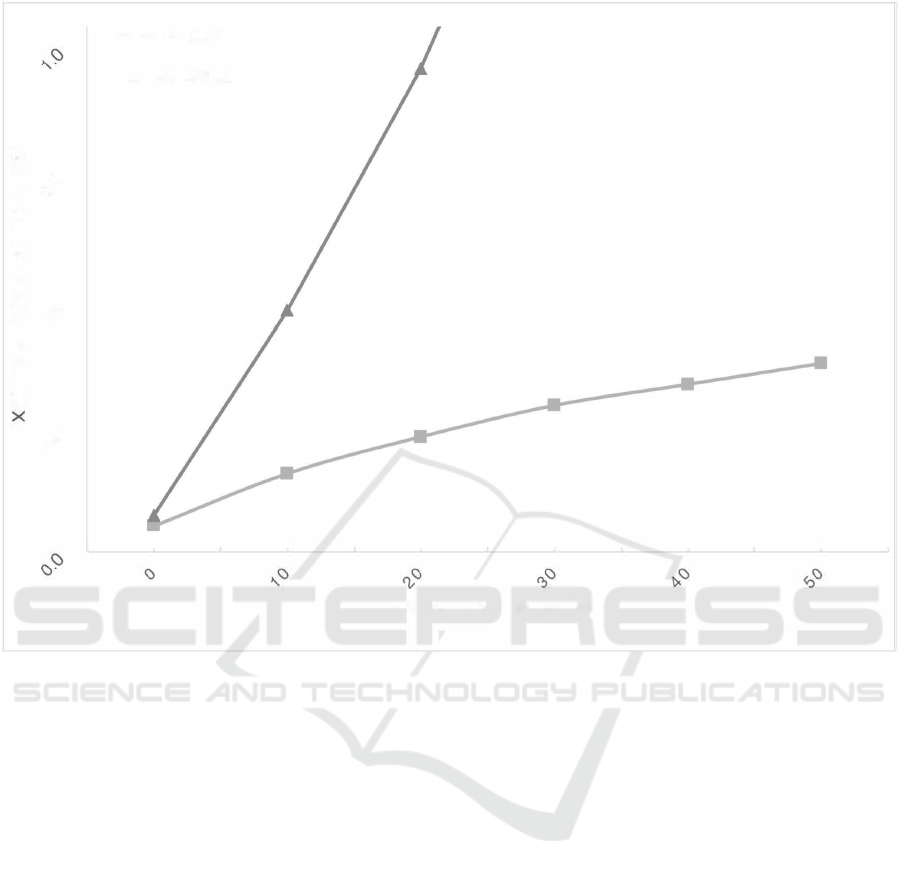
-di s CCP
dicExhau

6










�
z
0






NUMBER OF VARIABLES
Figure 6: Time needed to compute distance metrics with various numbers of constraints.
least performing one. This is mainly due to the ex-
ponential number of pairs that need to be computed
using this baseline method.
5 CONCLUSION AND FUTURE
WORK
We investigated the similarity between CCP-nets
which is of relevance when aggregating different
agents in recommender systems. The similarity is
computed based on either the Hamming distance (be-
tween the best outcomes of the related pair of CCP-
nets), or the number of CPT statements shared by
both CCP-nets. The first method, called disHCCP,
does require to solve both CCP-nets before comput-
ing the Hamming distance between the related opti-
mal solutions. This solving process requires an algo-
rithm of exponential time cost (Boutilier et al., 2004b;
Alanazi and Mouhoub, 2016). The second method,
called disCCP, consists of traversing both CCP-nets in
a topological order to compute the similarity based on
the number of identical orders in the related induced
graphs. An experimental study has been conducted in
order to assess the time performance of each method,
and the results favor disCCP.
In the near future, we plan to extend our definition
of similarity to other CCP-net variants for expressing
qualitative preferences. These include probabilistic
(Ahmed and Mouhoub, 2018) and constrained TCP-
nets (Zhang et al., 2015), partial CP-nets (Ahmed and
Mouhoub, 2018) and those considering genuine deci-
sions (Ahmed and Mouhoub, 2020).
We will also consider other graphical models for
representing preferences such as LP-trees (Li and
Kazimipour, 2018; Ahmed and Mouhoub, 2019),
GAI-nets (Gonzales and Perny, 2004), and those mod-
els for handling temporal information (Mouhoub and
Sukpan, 2008; Mouhoub and Liu, 2008).
REFERENCES
Ahmed, S. and Mouhoub, M. (2018). Constrained op-
timization with preferentially ordered outcomes. In
Tsoukalas, L. H., Gr
´
egoire,
´
E., and Alamaniotis, M.,
editors, IEEE 30th International Conference on Tools
ICAART 2022 - 14th International Conference on Agents and Artificial Intelligence
232

with Artificial Intelligence, ICTAI 2018, 5-7 Novem-
ber 2018, Volos, Greece, pages 307–314. IEEE.
Ahmed, S. and Mouhoub, M. (2019). Lexicographic pref-
erence trees with hard constraints. In Meurs, M.
and Rudzicz, F., editors, Advances in Artificial Intelli-
gence - 32nd Canadian Conference on Artificial Intel-
ligence, Canadian AI 2019, Kingston, ON, Canada,
May 28-31, 2019, Proceedings, volume 11489 of
Lecture Notes in Computer Science, pages 366–372.
Springer.
Ahmed, S. and Mouhoub, M. (2020). Conditional prefer-
ence networks with user’s genuine decisions. Comput.
Intell., 36(3):1414–1442.
Alanazi, E. and Mouhoub, M. (2016). Variable ordering and
constraint propagation for constrained cp-nets. Ap-
plied Intelligence, 44(2):437–448.
Alanazi, E., Mouhoub, M., and Zilles, S. (2020). The com-
plexity of exact learning of acyclic conditional pref-
erence networks from swap examples. Artif. Intell.,
278.
Balke, W.-T. and Wagner, M. (2003). Towards personalized
selection of web services. In WWW (Alternate Paper
Tracks), pages 20–24.
Bonnefon, J.-F., Shariff, A., and Rahwan, I. (2016). The
social dilemma of autonomous vehicles. Science,
352(6293):1573–1576.
Boutilier, C., Brafman, R. I., Domshlak, C., Hoos, H. H.,
and Poole, D. (2004a). Cp-nets: A tool for repre-
senting and reasoning withconditional ceteris paribus
preference statements. Journal of artificial intelli-
gence research, 21:135–191.
Boutilier, C., Brafman, R. I., Domshlak, C., Hoos, H. H.,
and Poole, D. (2004b). Preference-based constrained
optimization with cp-nets. Computational Intelli-
gence, 20(2):137–157.
Dalla Pozza, G., Pini, M. S., Rossi, F., and Venable, K. B.
(2011). Multi-agent soft constraint aggregation via se-
quential voting. In Twenty-Second International Joint
Conference on Artificial Intelligence.
Domshlak, C., H
¨
ullermeier, E., Kaci, S., and Prade, H.
(2011). Preferences in ai: An overview, artifical in-
telligence, 175 (7-8).
Goldsmith, J. and Junker, U. (2008). Preference handling
for artificial intelligence. AI Magazine, 29(4):9–9.
Gonzales, C. and Perny, P. (2004). Gai networks for utility
elicitation. KR’04, page 224–233. AAAI Press.
Lang, J. (2010). Graphical representation of ordinal pref-
erences: Languages and applications. In Interna-
tional Conference on Conceptual Structures, pages 3–
9. Springer.
Li, M. and Kazimipour, B. (2018). An efficient algorithm
to compute distance between lexicographic preference
trees. In IJCAI, pages 1898–1904.
Loreggia, A., Mattei, N., Rossi, F., and Venable, K. B.
(2018a). 18 value alignment via tractable preference
distance.
Loreggia, A., Mattei, N., Rossi, F., and Venable, K. B.
(2018b). A notion of distance between cp-nets. In
Proc. of AAMAS, pages 955–963.
Mohammed, B., Mouhoub, M., and Alanazi, E. (2015).
Combining constrained cp-nets and quantitative pref-
erences for online shopping. In International Confer-
ence on Industrial, Engineering and Other Applica-
tions of Applied Intelligent Systems, pages 702–711.
Springer.
Mouhoub, M. and Liu, J. (2008). Managing uncertain tem-
poral relations using a probabilistic interval algebra.
In 2008 IEEE International Conference on Systems,
Man and Cybernetics, pages 3399–3404.
Mouhoub, M. and Sukpan, A. (2008). Managing tempo-
ral constraints with preferences. Spatial Cognition &
Computation, 8(1-2):131–149.
Moussa, A. S. (2019). On learning and visualizing lexico-
graphic preference trees. University of North Florida.
Racharak, T., Suntisrivaraporn, B., and Tojo, S. (2016).
simπ: A concept similarity measure under an agent’s
preferences in description logic elh. In Proceedings
of the 8th International Conference on Agents and Ar-
tificial Intelligence - Volume 2: ICAART,, pages 480–
487. INSTICC, SciTePress.
Ricci, F., Rokach, L., and Shapira, B. (2011). Introduction
to recommender systems handbook. In Recommender
systems handbook, pages 1–35. Springer.
Rossi, F., Venable, K. B., and Walsh, T. (2004). mcp nets:
Representing and reasoning with preferences of mul-
tiple agents. In AAAI, volume 4, pages 729–734.
Wang, H., Wang, H., Guo, G., Tang, Y., and Zhang, J.
(2017). Measuring similarity of users with qualita-
tive preferences for service selection. Knowledge and
Information Systems, 51(2):561–594.
Xu, K. and Li, W. (2000). Exact phase transitions in random
constraint satisfaction problems. Journal of Artificial
Intelligence Research, 12:93–103.
Yager, R. (2001). Penalizing strategic preference manipu-
lation in multi-agent decision making. IEEE Transac-
tions on Fuzzy Systems, 9(3):393–403.
Zhang, S., Mouhoub, M., and Sadaoui, S. (2015). Integrat-
ing tcp-nets and csps: The constrained tcp-net (ctcp-
net) model. In 28th International Conference on In-
dustrial, Engineering and Other Applications of Ap-
plied Intelligent Systems, IEA/AIE 2015, Seoul, South
Korea, June 10-12, 2015, Proceedings, volume 9101
of Lecture Notes in Computer Science, pages 201–
211. Springer.
Constrained CP-nets Similarity
233