Prediction of Store Demands by Decision Trees and Recurrent Neural

Networks Ensemble with Transfer Learning

Nikica Peri

1 a

, Naomi-Frida Muniti

1 b

, Ivana Ba

sljan

1 c

and Vinko Le

1 d

Laboratory for Renewable Energy Systems, Faculty of Electrical Engineering and Computing,

University of Zagreb, Zagreb, Croatia

Keywords:

Multi Period VRP, Prediction of Delivery Capacities, Gradient Boosting Decision Trees, Recurrent Neural

Networks, Transfer Learning.

Abstract:

Simple vehicle routing problem (VRP) algorithms today achieve near-optimal solution and solve problems

with a large number of nodes. Recently, these algorithms are upgraded with additional constraints to respect an

increasing number of real-world conditions and, further on, adding a predictive character to the optimization.

A distinctive contribution lies in taking into account the predictions of orders that are yet to occur. Such

problems fall under time series approaches that are most often obtained using statistical methods or historical

data heuristics. Machine learning methods have proven to be superior to statistical methods in most of the

literature. In this paper, machine learning techniques for predicting the mass of total daily orders for individual

stores are further elaborated and tested on historical data of a local retail company. Among the tested methods

are Gradient Boosting Decision Tree methods (XGBoost and LightGBM) and methods of Recurrent Neural

Networks (LSTM, GRU and their variations using transfer learning). Finally, an ensemble of these methods is

performed, which provides the highest prediction accuracy. The ﬁnal models use the information on historical

order quantities and time-related slack variables.

1 INTRODUCTION

The Vehicle Routing Problem (VRP) is one of the

most studied topics when it comes to combinatorial

optimization and operations research. The goal of a

VRP is to enable orders to be delivered to the desired

locations in a desired time with the lowest possible

costs. Since the problem is very complex compu-

tationally (complexity is O(n!), where n is the total

number of locations), it is impossible to ﬁnd an opti-

mal solution for problems with a large number of lo-

cations in a limited time. Therefore, various methods

are developed to ﬁnd a suboptimal solution. Heuristic

and meta-heuristic methods based on local search are

most often used (Gillett and Miller, 1974), (Rochat

and Taillard, 1995), (Nagata and Br

aysy, 2009). More

recently a number of algorithms use deep reinforce-

ment learning (Nazari et al., 2018).

There are different variants of a VRP depend-

ing on what requirements it should meet during

https://orcid.org/0000-0002-2476-6305

https://orcid.org/0000-0002-8337-6251

https://orcid.org/0000-0001-9495-6342

https://orcid.org/0000-0003-1595-6016

optimization. Among established variants are Ca-

pacitated Vehicle Routing Problem (CVRP) intro-

duced in (Dantzig and Ramser, 1959) and Vehi-

cle Routing Problem with Time Windows (VRPTW)

elaborated in (Solomon, 1987). Recent research

often analyzes other variants such as Multidepot

Vehicle Routing Problem (MDVRP), (Lau et al.,

2010), Three-dimensional Loading Capacitated Ve-

hicle Routing Problem (3L-CVRP,) (Tarantilis et al.,

2009) or Pickup and Delivery Vehicle Routing Prob-

lem (PDVRP), (Chen and Fang, 2019). Additional

variants are often combined with CVRP and VRPTW

to better incorporate real-world requirements as e.g.

in (Wang et al., 2016). Despite many requirements

that are being considered in optimization, little atten-

tion is paid to the predictive component.

The Time Dependent Vehicle Routing Problem

(TDVRP) takes into account the time component to

avoid trafﬁc jams. The TDVRP consideres 3.06% of

VRP papers from the 2009-2015 period according to

(Braekers et al., 2016). The predictive component

that combines current orders with anticipated orders

for other days or shifts is used in even fewer VRP al-

gorithms. This variant is called Multi Period Vehicle

218

Peri

c, N., Muniti

c, N., Bašljan, I. and Leši

c, V.

Prediction of Store Demands by Decision Trees and Recurrent Neural Networks Ensemble with Transfer Learning.

DOI: 10.5220/0010802500003116

In Proceedings of the 14th International Conference on Agents and Artiﬁcial Intelligence (ICAART 2022) - Volume 3, pages 218-225

ISBN: 978-989-758-547-0; ISSN: 2184-433X

Routing Problem (MPVRP) and can be found in (Wen

et al., 2010) or (Mancini, 2016). The authors identify

variables where predictions should improve the exist-

ing state of VRP algorithms, especially in the last-

mile delivery. These are: i) prediction of the delivery

point time matrix (used for TDVRP), ii) prediction of

store (delivery point) activity, and iii) prediction of

the quantity of goods to be delivered (can be divided

into mass prediction and volume prediction). The TD-

VRP implies variable time matrices at different times

of the day, which also takes into account realistic traf-

ﬁc phenomena. Using these matrices, it is possible to

avoid trafﬁc jams in cities by sending vehicles mostly

to the outskirts of the city during heavy trafﬁc, and to

the city center when there is less trafﬁc. Predictions

of store (delivery point) activity allow the algorithm to

better schedule locations visits so that a delivery ve-

hicle visits a speciﬁc location fewer times. These pre-

dictions are beneﬁcial for a VRP with a time horizon,

and if orders can be postponed for other days. Pre-

diction of the quantity of goods to be delivered is also

essential in this case. Estimating the quantity needed

to be delivered over the time horizon is important for

determination of how many vehicles and what types

of vehicles are needed to deliver all orders. If nec-

essary, it is possible to postpone deliveries to another

day or to deliver in advance, which reduces the need

for borrowing external vehicles or overtime work and

thus the total operating costs.

In this paper, methods for predicting the mass of

goods to be delivered are compared. Statistical mod-

els such as Autoregressive Integrated Moving Aver-

age (ARIMA) and some of its more advanced vari-

ations are mostly used for similar time series pre-

dictions (Zhang, 2003), (Pavlyuk, 2017). With the

growing popularity of machine learning, new meth-

ods have been developed that are superior in accu-

racy to such statistical methods. (Siami-Namini et al.,

2018). Machine learning methods are used for simi-

lar applications in: (Anzar, 2021), (Mackenzie et al.,

2019) and (Fu et al., 2016). For retail sales series

that are often found as non-linear problems, due to the

seasonality, basic statistical models and linear models

of machine learning are unable to solve such prob-

lems with a higher accuracy. Therefore, it is rec-

ommended to experiment with advanced forecasting

methods such as Neural Networks or Gradient Boost-

ing Methods (Wanchoo, 2019). In further research, it

is also worth to notice that those two models mostly

perform better than other time series and regression

techniques, including cases related to store demands

(Hod

c et al., 2019).

The methods tested are separated into two groups:

Gradient Boosting Decision Tree (GBDT) and Re-

current Neural Networks (RNN). Among the GBDT

methods, Extreme Gradient Boosting (XGBoost) and

Light Gradient Boosting Method (LightGBM) are

considered. Among the RNN methods, Long Short-

Term Memory (LSTM), Gated Recurrent unit (GRU)

are tested, and these two methods with transfer learn-

ing are considered as a special cases. The same meth-

ods can be used after re-tuning of hyperparameters to

predict the time matrix and predict the activity of the

stores.

This paper ﬁrst brieﬂy presents all the methods

used in Section II. Section III describes the observed

dataset. Utilized approaches are presented in Section

IV. Data pre-processing, common to all models, is de-

scribed ﬁrst, followed by the selection of hyperparam-

eters and post-processing. Section V presents the re-

sults. In Section VI, a conclusion is given.

2 METHODOLOGY

The GBDT and RNN methods listed in the introduc-

tion are used to predict the mass of goods to be deliv-

ered. These methods are described below.

2.1 Gradient Boosting Decision Tree

The GBDT is a widely used machine learning al-

gorithm thanks to its efﬁciency and interpretability.

The model consists of an ensemble of weak mod-

els (decision trees) that through the epochs with the

use of previous models become more accurate and to-

gether give better predictions than individual models.

These predictions, due to a large number of ”weak”

models, give robustness to the common model. Ex-

treme Gradient Boosting (Chen and Guestrin, 2016)

and LightGBM Method (Ke et al., 2017) are currently

among the most successful GBDT implementations.

Compared to standard GBDT, XGBoost provides a

parallel tree boosting to increase speed, uses regu-

larized model and implements Dropouts meet mul-

tiple Additive Regression Trees (DART) to reduce

overﬁtting, Newton Boosting to converge faster, etc.

The LightGBM algorithm has some changes in addi-

tion to those XGBoost has. The changes are: i) the

Histogram-Based Gradient Boosting algorithm which

increases the execution speed, ii) leaf-wise (best-ﬁrst)

tree growth instead of level-wise tree growth in XG-

Boost, iii) support for categorical features, etc. The

disadvantage is a large number of hyperparameters,

which makes it difﬁcult to do a detailed grid search.

Prediction of Store Demands by Decision Trees and Recurrent Neural Networks Ensemble with Transfer Learning

219

2.2 Recurrent Neural Networks

The application of Recurrent Neural Networks has in-

creased signiﬁcantly with the increase in computer

processing power in recent years. The RNNs are se-

lected here because of the chain structure correspond-

ing to time series predictions. The main disadvantage

of classical RNNs is the vanishing gradient problem,

which is mitigated by recently established methods

such as LSTM (Hochreiter and Schmidhuber, 1997)

and GRU (Chung et al., 2014). The LSTM networks

solve this problem using three regulators (gates): for-

get, input and output. The GRU networks are intro-

duced as a variation of LSTM in which the number of

gates is reduced to 2: reset and update. This results in

higher speed and fewer neurons in a single cell, mak-

ing the GRU networks easier to prevent overﬁtting.

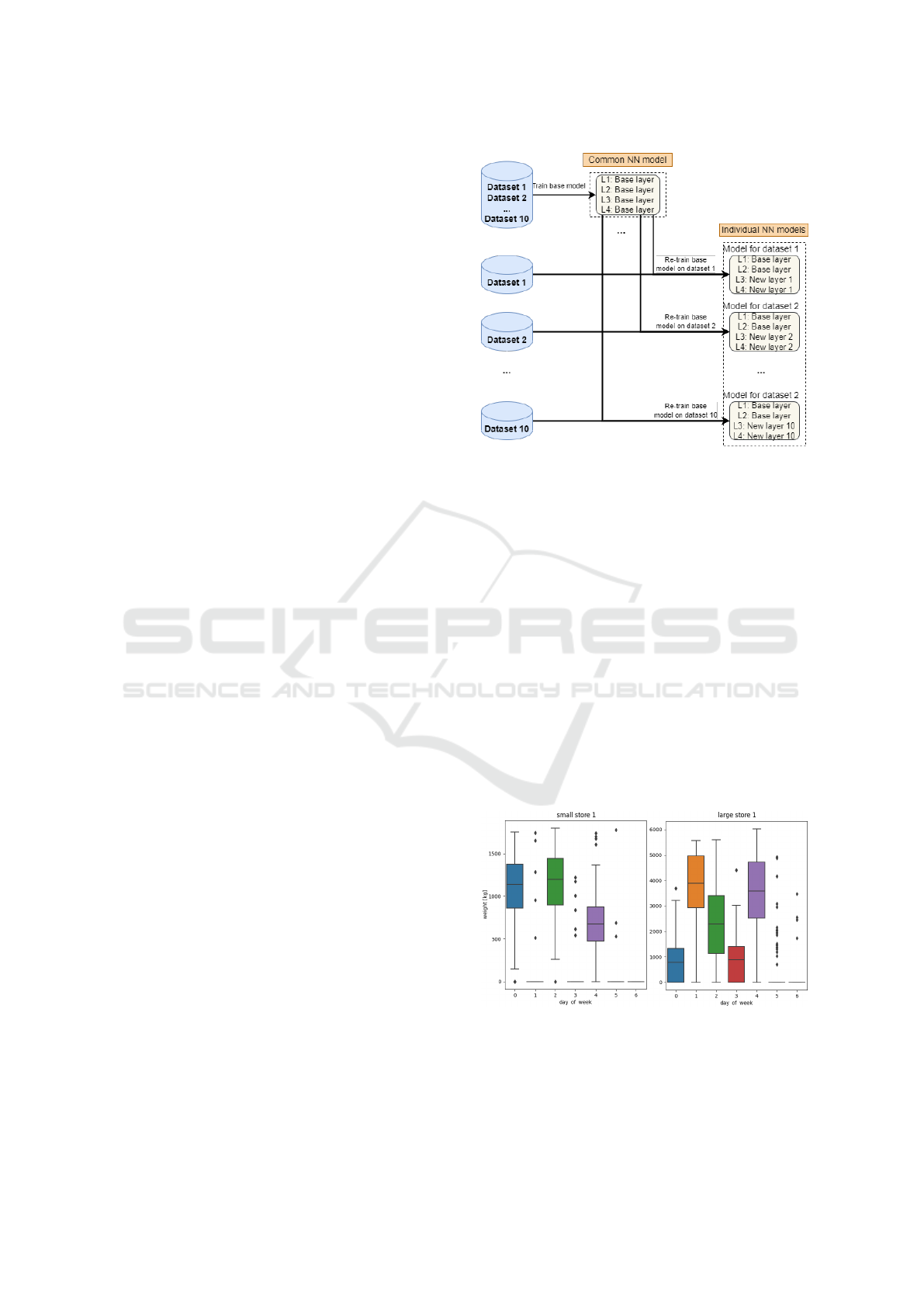
2.3 Transfer learning

Transfer learning is a method where the model is

ﬁrst trained using one, usually larger dataset, and

then reused and adapted to another, usually smaller

dataset. Although more commonly used in classiﬁca-

tion problems, transfer learning has some applications

in time series prediction (He et al., 2019), (Chaura-

sia and Pal, 2020). According to (Tan et al., 2018),

transfer learning is separated into four categories:

instances-based, mapping-based, network-based and

adversarial-based. The approach used in this paper

is network-based transfer learning. This is applica-

ble when multiple similar datasets relating to individ-

ual units (stores in this paper) are available. First, a

common base model is generated that is trained on all

datasets. Most of the hidden layers of the neural net-

work remain from this model, and the last layers are

then re-trained on individual sets. In this way, each

individual set has own prediction model while the ini-

tial layers are the same for all, and the last layers are

speciﬁc to each of the individual sets. The described

approach is shown in Fig. 1.

3 DATASET

The presented predictions are generated from a histor-

ical dataset of a retail company that owns over 1000

delivery locations, of which over 200 are in the con-

sidered city. Most locations relate to stores and ware-

houses. These stores are separated into large, medium

and small categories based on the daily turnover of

goods and the type of goods in the store. The com-

pany also owns a heterogeneous ﬂeet of delivery vehi-

cles. These vehicles transport goods from warehouses

Figure 1: Network based transfer learning structure for 10

individual sets.

to stores. Due to the access restrictions of some trucks

and with the aim of quality planning of the MDVRP, it

is important that the stores are observed individually.

Also, groups of stores differ in some ordering habits,

so most large stores have orders every work day, while

small ones usually order demands 2-3 times a week.

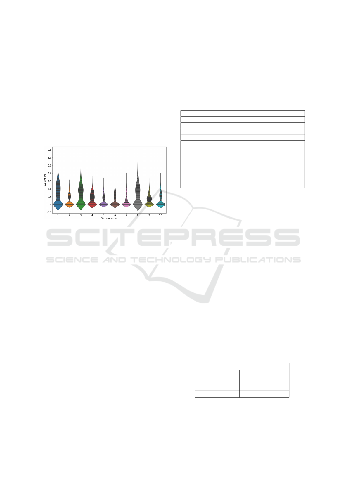
This is evident from Fig. 2, which on the left shows

mass distribution of demands for small store 1 over

the days of the week, and for large store 1 on the right.

Therefore, 10 small, 10 medium and 10 large stores

are selected to test the machine learning models. For

small stores, data processing, tables and predictions

are presented in detail for elaboration and presenta-

tion purpose and while for medium and large stores,

only the ﬁnal prediction results are shown for meth-

ods scale-up purpose. The data processing procedure

is the same for all 3 types of stores.

Figure 2: Distribution of mass in kilograms by days of week

for small store 1 and big store 1.

The original dataset refers to 2018 and 2019 (730

days) and is structured as a list of orders. Each or-

der corresponds to a speciﬁc date and mass of goods.

ICAART 2022 - 14th International Conference on Agents and Artiﬁcial Intelligence

220

The dataset is restructured into a 2D array where the

columns represent different stores, and each row cor-

responds to a single day. The distribution by mass of

daily orders for each small store is shown in Fig. 3.

The x-axis shows small stores sorted by indices (from

1 to 10), and the y-axis shows the mass that stores

ordered. The wider part of the graph for a particu-

lar store indicates a larger number of orders of simi-

lar mass over the observed time period. For example,

store 5 has fewer days with order deliveries compared

to store 8. Store 1 has an approximately normal dis-

tribution if we exclude non-delivery days, compared

to store 7.

Figure 3: Distribution of mass in tons by daily orders for

each small store.

4 UTILIZED APPROACHES

In order to increase the quality of predictions, the

dataset is preprocessed and inputs obtained by fea-

ture engineering are tested. The already mentioned 6

models with appropriate hyperparameters and an en-

semble of them is tested, and then the results are post

processed. In the sequel, common models notation is

used for transfer learning models from the upper part

of Fig. 1 and individual models refers to XGBoost,

LightGBM, LSTM, GRU, and the lower part of Fig. 1.

4.1 Preprocessing and Feature

Engineering

As mentioned before, the dataset is separated into

three smaller datasets containing orders for 10 small,

10 medium and 10 large stores from 2018 and 2019.

The reason for the separation into categories is that

common models use data similar to individual mod-

els because stores of the same size have similar habits

of ordering goods. The input data for all 6 models

are the same and consist of the variables listed in Ta-

ble I. The common models for ﬁrst store s

have s

i, j

and w

as the inputs, and the inputs of the individu-

als model are s

1, j

, d

and w

. The inputs contain data

from the last 14 days (t

· h), by which the model pre-

dicts demands for the next day (t

· f ). The variable s

is used to designate days in a week, with demands for

all 10 stores.

Table 1: Models inputs, outputs and common hyperparam-

eters.

Variable and values Description

store designation, i ∈{1,...,10}

i,j

∈{1,...,m

max

} historical store demands,

i ∈{1,...,10}, j ∈{1,...,h}

∈{1,...,7} day of week, j ∈{1,...,h}

∈{0, 1} working or non-working day,

j ∈{1,...,h}

i,j

∈{1,...,m

max

} predictions of store demands,

i ∈{1,...,10}, j ∈{1,...,f }

m > 0 Store demands mass in kg

= 1 day Predictions and data resolution

h Amount of historical input values

f Amount of future values to predict

It is observed that stores of similar size have sim-

ilar behavior. Small stores usually have 1-3 orders

per week, while large ones have orders every work-

ing day. In some stores, a change in the customer

habits is noticeable, e.g., a change in the usual or-

dering days from Tuesday and Thursday to Monday

and Friday. In some, an increase or decrease in the

number of orders is evident during the observed pe-

riod, which is caused by a change in the turnover of

the store, and consequently by the number of workers

in it. Among the noticeable deviations are also sin-

gle change of order day, different behavior before the

holidays, etc. Since individual models often do not

have information to learn such behavior changes well

enough, common models are introduced in which

such behavior changes are learned from other stores.

In order not to create bias, common models for small,

medium and large stores are separated according to

the average mass of demands in one day:

i,avg

∑

730

j=1

i, j

730

, (1)

as shown in Table II.

Table 2: Separation of stores by size.

Stores daily demands mass [kg]

size min max average

small 0 500 242.9

medium 500 1250 824.6

large 1250 - 3704.4

The correlation matrix of input variables is shown

in Fig. 4 for the category of small stores. The order

of the variables was chosen according to the corre-

Prediction of Store Demands by Decision Trees and Recurrent Neural Networks Ensemble with Transfer Learning

221

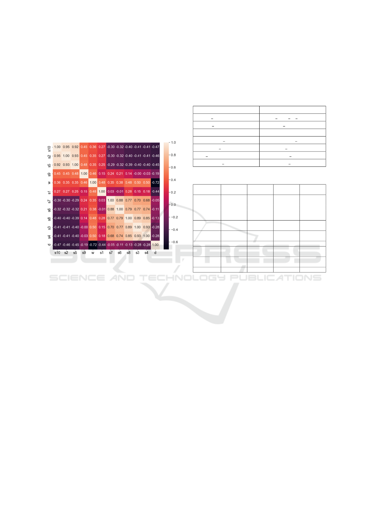
lation value to make clusters of similar stores more

noticeable. As expected, w has a positive and d nega-

tive correlation with all stores. Very high correlations

should be noted: s

, s

and s

group, s

, s

and s

group and s

to s

. These groups of stores have com-

mon ordering habits (mostly ordering on the same day

of the week), which makes the common model more

adjusted to them. The variables d and w are mainly

used to identify the days with orders, which is evident

from their correlations (both have similar correlations

to each of the stores, especially w).

Figure 4: Correlation matrix of all models inputs.

The insertion of a rolling average on the input and

a slack variable that gives 1 on days when there is

a demand, and 0 when there is no demand, is also

tested. However, these variables did not prove to be

beneﬁcial for the models.

In Fig. 3, several outliers can be seen. They are

corrected using the 2σ rule. When calculating out-

liers, days without deliveries are not considered, and

too big values of demands are corrected using the for-

mula:

i, j

= max(s

i, j

, s

i,avgp

+ 2 · s

i,stdp

+ 0.1 · s

i, j

), (2)

where s

i,avgp

and s

i,stdp

are average and standard de-

viation of positive s

i, j

values. In this way, an average

of 3 outliers per store is corrected.

Datasets in RNN models are separated chronolog-

ically into parts for training, validation and test in the

ratio of approximately 60%-20%-20%, and in GBDT

methods they are separated into parts for training and

test in the ratio 80%-20%. For RNN methods, Min-

Max scaler with [0, 1] limits is used.

4.2 Hyperparameters Selection

After selecting inputs, prediction models are created.

Grid search is applied to all models. The best ob-

tained hyperparameter values for the XGBoost and

LightGBM models are shown in Table III. Table IV

shows parameters for LSTM, GRU, LSTM with trans-

fer learning and GRU with transfer learning.

Table 3: XGBoost and LightGBM hyperparameters.

XGBoost LightGBM

reg lambda = 0.15 min data in leaf = 20

reg alpha = 0.004 num leaves = 10

subsample = 0.4 subsample = 0.7

colsample bytree = 0.4 subsample freq = 5

max depth = 4 max depth = 5

n estimators = 500 colsample bytree = 0.7

learning rate = 0.01 learning rate = 0.04

Table 4: RNN methods hyperparameters.

Hyper- LSTM GRU LSTM GRU

parameter transfer transfer

LSTM(40) GRU(40) LSTM(40) GRU(40)

Dropout(0.2) Dropout(0.1) Dropout(0.2) Dropout(0.2)

Layers LSTM(40) GRU(25) LSTM(40) GRU(40)

Dropout(0.2) Dropout(0.1) Dropout(0.2) Dropout(0.2)

LSTM(1) GRU(1) LSTM(1) GRU(1)

Transfer lear- / / LSTM(25) GRU(25)

ning layers LSTM(1) GRU(1)

Loss RMSE RMSE RMSE RMSE

functions MAE* MAE* MAE* MAE*

Optimizer Adam Adam Adam Adam

Learning rate 0.003 0.003 0.002 0.002

0.001** 0.001**

Epochs 200 200 200 200

30** 30**

Batch size 50 50 50 50

Used for evaluation only, not in training

Refers to the learning of an individual part of a model

4.3 Post-processing and Ensemble

Model

After selecting the hyperparameters, 6 models are

trained and predictions are obtained. RNN prediction

values are scaled back to the original range to be com-

parable to GBDT methods. After that, all predictions

values less than a quarter of the mean value are sat-

urated to 0. An ensemble of the four most accurate

models has been created, which gives the weighted

average of the output of these four models at the out-

put. The predictions of the ensemble model are cal-

culated by:

i, j(e)

= 0.1p

i, j(1)

+0.2p

i, j(4)

+0.25p

i, j(5)

+0.45p

i, j(6)

(3)

where p

i, j(e)

is ensemble prediction, p

i, j(1)

is XG-

Boost prediction, p

i, j(4)

is GRU prediction, p

i, j(5)

LSTM with transfer learning prediction and p

i, j(6)

GRU with transfer learning prediction.

ICAART 2022 - 14th International Conference on Agents and Artiﬁcial Intelligence

222

5 EXPERIMENT AND RESULTS

5.1 Small Stores

All models are tested on test sets for 10 small stores.

Table V shows the results. The upper values for

each store refer to Root Mean Squared Error (RMSE)

and the lower values to Mean Absolute Error (MAE).

RMSE is observed as the main metric. In addition to

the results for all 10 stores individually, average errors

and the time in seconds required to learn the model for

all 10 stores are added.

Table 5: Comparison of prediction accuracy for small stores

category.

store XG- Light- LSTM GRU LSTM GRU ens-

Boost GBM transfer transfer amble

s1 265.0 271.2 256.6 277.2 258.1 264.0 252.2

151.8 151.8 140.1 136.2 140.2 142.3 135.6

s2 140.2 145.3 142.1 136.1 134.4 126.0 127.1

67.2 69.7 58.3 55.3 61.0 56.8 57.9

s3 341.7 352.8 329.2 335.8 338.5 305.2 307.3

198.2 204.0 187.7 177.9 178.2 174.3 168.8

s4 188.8 196.9 197.9 181.0 172.5 174.2 166.9

101.9 109.3 127.3 95.8 94.1 98.2 92.8

s5 119.5 129.1 127.0 121.8 93.9 102.5 98.3

53.1 58.0 52.9 55.2 43.1 48.4 46.1

s6 171.7 184.4 224.5 168.8 169.5 161.3 156.0

82.2 89.8 124.7 82.7 75.8 81.0 77.6

s7 108.9 117.2 141.1 94.7 98.6 89.3 88.9

44.8 50.7 88.3 45.5 43.2 42.3 41.7

s8 307.7 345.6 287.1 303.6 354.4 302.1 301.7

153.6 176.1 144.9 158.4 179.5 158.0 157.9

s9 175.7 179.3 189.4 171.4 175.3 159.7 160.6

95.8 95.1 103.3 101.9 95.0 86.1 89.6

s10 150.2 151.5 159.1 151.0 129.4 134.2 132.6

72.7 74.8 68.0 73.4 57.8 64.9 62.9

avg. 197.0 207.3 206.4 194.1 192.5 181.9 179.2

102.1 107.9 109.6 98.2 96.8 95.2 93.1

Time

4.9 1.8 255.6 196.7 169.7 140.7 512.0

Upper values in the rows denote RMSE, lower are for MAE

Table shows that the XGBoost method gives bet-

ter accuracy than LightGBM, and the GRU is more

accurate than LSTM, according to RMSE and MAE.

Two models using transfer learning compared to the

same methods without transfer learning achieve sig-

niﬁcant progress: 9% for LSTM and 5% for GRU.

Transfer learning brings the greatest progress in s

and s

stores, which together with s

make up the

group of stores with the highest correlations (Fig. 4).

It is concluded that, by increasing the number of ob-

served stores, transfer learning could bring an addi-

tional advantage in the accuracy of predictions. In

that case, instead of separating stores according to the

number of deliveries, it would be good to use some

more advanced form of clustering. The ensemble of

4 best methods provides the best results as expected,

2% better than GRU with transfer learning.

Part of the predictions from Table V are also

shown in Fig. 5. The ﬁgure shows the 45 days of pre-

dictions given by the algorithm on the test set of the

s3 store. Predictions from the ﬁgure omit described

post-processing (saturation to zero) for the purpose

of better illustration. During the usual, steady-state,

schedule of order days, all models give similar predic-

tions. A higher difference in accuracy occurs on days

when the order schedule changes rapidly. The sched-

ule has changed on 8.10.2019., which greatly inﬂu-

enced the predictions for the following days. Models

with XGBoost and LightGBM do not change the be-

havior much, LSTM partially changes the behavior,

and the other 3 models adapt more to the new behav-

ior, especially the GRU model with transfer learning.

Precisely, such situations are the biggest advantage of

transfer learning methods. The disadvantage of these

methods may be the learning speed at which XGBoost

and LightGBM are far better. Nevertheless, all tested

algorithms are fast enough for this application. Ap-

plications such as TDVRP in which predictions are

made for each of the two store combinations should

also consider the speed component.

5.2 All Stores

The algorithms are tested on a set of 10 medium and a

set of 10 large stores. Table VI lists RMSE and MAE

for all 3 types of stores. The results for medium and

large stores are similar to those for the small ones.

Predictions with GBDT and RNN methods have sim-

ilar results, and transfer learning brings advances in

models with an emphasis on smaller stores. The best

results are obtained using an ensemble of a few meth-

ods. The results of the ensemble of methods are com-

pared with a model that copies occurrences from 7

days ago for working days and predicts 0 for non-

working days. A 57% lower loss is obtained for small

stores, 60% lower for medium, and 54% for large

ones. Such persistence model gives RMSE = 412.4kg

and MAE = 221.8kg for all 10 observed test datasets

of 4 months for the small stores, i.e. the ensemble

approach provides 57% improvement in prediction

accuracy. For the medium and the large stores, en-

semble provides 60% and 54% improvement, respec-

tively, while the most evident improvement is during

rapid changes in stores demand. This is of great ben-

eﬁt to Multi Period VRP because prediction of total

weight of order directly affects the number of vehi-

cles, overtime hours, but also the total cost of deliv-

ery.

Prediction of Store Demands by Decision Trees and Recurrent Neural Networks Ensemble with Transfer Learning

223

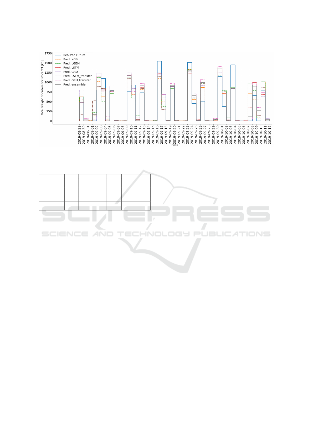
Figure 5: Comparison of prediction accuracy for all tested methods.

Table 6: Comparison of prediction accuracy for all stores

categories.

stores XG- Light- LSTM GRU LSTM GRU ens-

size Boost GBM transfer transfer amble

small 197.0 207.3 206.4 194.1 192.5 181.9 179.2

102.1 107.9 109.6 98.2 96.8 95.2 93.1

medi- 645.1 660.1 688.5 639.6 654.1 638.7 616.8

um 346.5 345.4 355.6 330.9 338.3 329.3 322.2

large 2398 2385 2470 2467 2621 2368 2339

1670 1647 1692 1699 1832 1660 1647

Upper values in the rows denote RMSE, lower are for MAE

6 CONCLUSION

In this paper, machine learning methods for predic-

tion of delivery capacities in last-mile logistics are

tested. These predictions are important to enable

the use of Multi Period VRP. Predictions are gener-

ated using Gradient Boosting Decision Tree methods

(XGBoost and LightGBM) and methods of Recurrent

Neural Networks (LSTM, GRU and their variations

using transfer learning). Real historical datasets are

used, divided into 3 categories according to store size.

At the inputs of all algorithms are the historical mass

values of the store order and slack variables depict-

ing working days and day of the week. Preprocess-

ing and post-processing are applied. Among the men-

tioned methods, GRU with transfer learning proves

to be the most accurate. Transfer learning generally

brings an improvement over the same metrics without

transfer learning, GRU is more accurate than LSTM,

and XGBoost is more accurate than LightGBM. RNN

methods are more accurate than GBDT methods for

small and medium-sized stores where orders are more

volatile, and GBDT methods are more accurate in

large stores. Eventually an ensemble of these methods

is generated which, as expected, gives the most accu-

rate predictions (2% compared to GRU with transfer

learning and 57% compared to persistence model).

ACKNOWLEDGEMENTS

This work has been supported by the European

Union from the European Regional Development

Fund via Operational Programme Competitiveness

and Cohesion 2014-2020 for Croatia through the

project Research and development of a uniﬁed sys-

tem for logistic and transport optimisation - Collab-

orative Elastic and Green Logistics - CEGLog (grant

KK.01.2.1.02.0081). The authors would like to thank

GDi Group for their collaboration.

REFERENCES

Anzar, T. (2021). Forecasting of Daily Demand’s Order Us-

ing Gradient Boosting Regressor BT - Progress in Ad-

vanced Computing and Intelligent Engineering. pages

177–186, Singapore. Springer Singapore.

Braekers, K., Ramaekers, K., and Van Nieuwenhuyse, I.

(2016). The vehicle routing problem: State of the art

classiﬁcation and review. Computers & Industrial En-

gineering, 99:300–313.

Chaurasia, V. and Pal, S. (2020). Application of machine

learning time series analysis for prediction COVID-19

pandemic. Research on Biomedical Engineering.

Chen, R. M. and Fang, P. J. (2019). Solving Vehicle Routing

Problem with Simultaneous Pickups and Deliveries

Based on A Two-Layer Particle Swarm optimization.

In 2019 20th IEEE/ACIS International Conference

on Software Engineering, Artiﬁcial Intelligence, Net-

ICAART 2022 - 14th International Conference on Agents and Artiﬁcial Intelligence

224

working and Parallel/Distributed Computing (SNPD),

pages 212–216.

Chen, T. and Guestrin, C. (2016). XGBoost: A scalable tree

boosting system. Proceedings of the ACM SIGKDD

International Conference on Knowledge Discovery

and Data Mining, 13-17-August-2016:785–794.

Chung, J., Gulcehre, C., Cho, K., and Bengio, Y. (2014).

Empirical Evaluation of Gated Recurrent Neural Net-

works on Sequence Modeling. pages 1–9.

Dantzig, G. B. and Ramser, J. H. (1959). The Truck Dis-

patching Problem. Management Science, 6(1):80–91.

Fu, R., Zhang, Z., and Li, L. (2016). Using LSTM and

GRU neural network methods for trafﬁc ﬂow predic-

tion. In 2016 31st Youth Academic Annual Conference

of Chinese Association of Automation (YAC), pages

324–328.

Gillett, B. E. and Miller, L. R. (1974). A Heuristic Algo-

rithm for the Vehicle-Dispatch Problem. Operations

Research, 22(2):340–349.

He, Q., Pang, P. C.-I., and Si, Y. W. (2019). Transfer Learn-

ing for Financial Time Series Forecasting. pages 24–

36.

Hochreiter, S. and Schmidhuber, J. (1997). Long Short-

Term Memory. Neural Computation, 9(8):1735–1780.

Hod

c, K., Hasi

c, H., Cogo, E., and Juri

Z. (2019).

Warehouse Demand Forecasting based on Long Short-

Term Memory neural networks. In 2019 XXVII Inter-

national Conference on Information, Communication

and Automation Technologies (ICAT), pages 1–6.

Ke, G., Meng, Q., Finley, T., Wang, T., Chen, W., Ma,

W., Ye, Q., and Liu, T. Y. (2017). LightGBM: A

highly efﬁcient gradient boosting decision tree. Ad-

vances in Neural Information Processing Systems,

2017-December(Nips):3147–3155.

Lau, H. C. W., Chan, T. M., Tsui, W. T., and Pang,

W. K. (2010). Application of Genetic Algorithms to

Solve the Multidepot Vehicle Routing Problem. IEEE

Transactions on Automation Science and Engineer-

ing, 7(2):383–392.

Mackenzie, J., Roddick, J. F., and Zito, R. (2019). An Eval-

uation of HTM and LSTM for Short-Term Arterial

Trafﬁc Flow Prediction. IEEE Transactions on Intel-

ligent Transportation Systems, 20(5):1847–1857.

Mancini, S. (2016). A real-life Multi Depot Multi Pe-

riod Vehicle Routing Problem with a Heterogeneous

Fleet: Formulation and Adaptive Large Neighborhood

Search based Matheuristic. Transportation Research

Part C: Emerging Technologies, 70:100–112.

Nagata, Y. and Br

aysy, O. (2009). Edge Assembly based

Memetic Algorithm for the Capacitated Vehicle Rout-

ing Problem. Networks, 54:205–215.

Nazari, M., Oroojlooy, A., Tak

c, M., and Snyder, L. V.

(2018). Reinforcement learning for solving the vehi-

cle routing problem. Advances in Neural Information

Processing Systems, 2018-Decem:9839–9849.

Pavlyuk, D. (2017). Short-term Trafﬁc Forecasting Using

Multivariate Autoregressive Models. Procedia Engi-

neering, 178:57–66.

Rochat, Y. and Taillard,

E. D. (1995). Probabilistic diversi-

ﬁcation and intensiﬁcation in local search for vehicle

routing. Journal of Heuristics, 1(1):147–167.

Siami-Namini, S., Tavakoli, N., and Namin, A. S. (2018).

A Comparison of ARIMA and LSTM in Forecast-

ing Time Series. In 2018 17th IEEE International

Conference on Machine Learning and Applications

(ICMLA), pages 1394–1401.

Solomon, M. M. (1987). Algorithms for the Vehicle Rout-

ing and Scheduling Problems with Time Window

Constraints. Operations Research, 35(2):254–265.

Tan, C., Sun, F., Kong, T., Zhang, W., Yang, C., and Liu,

C. (2018). A Survey on Deep Transfer Learning BT

- Artiﬁcial Neural Networks and Machine Learning –

ICANN 2018. pages 270–279, Cham. Springer Inter-

national Publishing.

Tarantilis, C. D., Zachariadis, E. E., and Kiranoudis, C. T.

(2009). A Hybrid Metaheuristic Algorithm for the

Integrated Vehicle Routing and Three-Dimensional

Container-Loading Problem. IEEE Transactions on

Intelligent Transportation Systems, 10(2):255–271.

Wanchoo, K. (2019). Retail Demand Forecasting: a Com-

parison between Deep Neural Network and Gradient

Boosting Method for Univariate Time Series. In 2019

IEEE 5th International Conference for Convergence

in Technology (I2CT), pages 1–5.

Wang, J., Zhou, Y., Wang, Y., Zhang, J., Chen, C.

L. P., and Zheng, Z. (2016). Multiobjective Vehicle

Routing Problems With Simultaneous Delivery and

Pickup and Time Windows: Formulation, Instances,

and Algorithms. IEEE Transactions on Cybernetics,

46(3):582–594.

Wen, M., Cordeau, J.-F., Laporte, G., and Larsen, J.

(2010). The dynamic multi-period vehicle rout-

ing problem. Computers & Operations Research,

37(9):1615–1623.

Zhang, G. (2003). Time series forecasting using a hybrid

ARIMA and neural network model. Neurocomputing,

50:159–175.

Prediction of Store Demands by Decision Trees and Recurrent Neural Networks Ensemble with Transfer Learning

225