A Constraint Programming Model for the Scheduling Problem with

Flexible Maintenance under Human Resource Constraints

Meriem Touat

1,2

, Belaid Benhamou

and Fatima Benbouzid-Si Tayeb

Ecole Sup

erieure des Sciences Appliqu

ees Alger (ESSA-Alger), BP 474 Place des Martyrs, Alger 16001, Algeria

Laboratoire des M

ethodes de Conception des Syst

emes (LMCS), Ecole Nationale Sup

erieure d’Informatique (ESI),

BP 68M 16309 Oued-Smar Alger, Algeria

Laboratoire LSIS, Domaine Universitaire de Saint-J

ome, Batiment Polytech,

Universit

e Aix-Marseille, Avenue Escadrille Normandie-Niemen, 13397 Marseille Cedex 20, France

Keywords:

Single Machine Scheduling, Flexible Maintenance Planning, OPL, Constraints Programming, Human

Resource Constraints.

Abstract:

In this work, we tackle the scheduling problem that considers both production and ﬂexible preventive main-

tenance on a single machine where the human resource constraints (the availability and the competence) are

taken into account. We propose a mathematical formulation for the problem that is expressed in the constraint

programming (CP) paradigm as a set of constraints. This CP modeling had been implemented using Ilog CP

Optimizer. Experiments were ﬁrst carried out on small instances to compare our CP implementation with that

one carried out in Mixed Integer Linear Program programming (MILP) presented in (Touat et al., 2021), then

the CP implementation had been tested on large instances and encouraging results were obtained.

1 INTRODUCTION

In this work, we deal with the single machine schedul-

ing problem with unavailability intervals due to the

preventive maintenance activities that could be pe-

riodic or ﬂexible. In theory, this kind of problems

have been proved to be NP-hard (Lee and Liman,

1992). To be solved, both exact and heuristic meth-

ods have been proposed in the literature. Indeed, sev-

eral mathematical modeling have been developed ac-

cording to the constraints taken into account ((Chen,

2008), (Cui and Lu, 2014), (Liu et al., 2015), (Yang

et al., 2011), (Mashkani and Moslehi, 2016)). How-

ever, given the high computational complexity of the

problem, exact algorithms could solve only small in-

stances in practice. Therefore, speciﬁc heuristics and

meta-heuristics have been extensively used to solve

larger instances of this problem ((Chen, 2008), (Low

et al., 2010), (Luo et al., 2015), (Yang et al., 2011),

(Zammori et al., 2014), (Yazdani et al., 2017)).

A new and more realistic single machine prob-

lem is introduced in works (Touat et al., 2017), (Touat

et al., 2018) and (Touat et al., 2021). In order to re-

ﬂect the reality of production shops, the authors as-

sumed that maintenance activities must be done by

human resources, characterized by a competence lev-

els and qualiﬁcations allowing them or not to execute

the maintenance activities with different durations. In

addition, these human resources are not available per-

manently, but in speciﬁed intervals that assess the fea-

sibility or not of the resulting schedules. First, a ge-

netic algorithm is proposed in (Touat et al., 2017) to

solve the problem in the uncertain context. Further,

both an exact method expressed as a Mixed Integer

Linear Program (MILP) and a metaheuristic are pro-

posed in (Touat et al., 2021) to deal with, respectively,

small and large instances of the problem. The exact

method is solved using the Ilog IBM Cplex, while

the metaheuristic is inspired from the Guided Local

Search method (GLS).

In addition to exact methods that are based on in-

teger programming (IP) and mixed integer linear pro-

gramming (MILP) formulations, the Constraint Pro-

gramming paradigm (CP) framework had been widely

applied to solve the scheduling problems. The com-

mercial solver IBM Ilog CP Optimizer that is used to

solve CP formulations, is a very known system in the

literature (Laborie et al., 2018). This solver is ded-

icated to ﬁnd optimal solutions, and when it is not

able to produce a such solution, it produces a good

quality solution in a reasonable amount of time. Fur-

thermore, the OPL (Optimization Programming Lan-

Touat, M., Benhamou, B. and Tayeb, F.

A Constraint Programming Model for the Scheduling Problem with Flexible Maintenance under Human Resource Constraints.

DOI: 10.5220/0010800700003116

In Proceedings of the 14th International Conference on Agents and Artiﬁcial Intelligence (ICAART 2022) - Volume 3, pages 195-202

ISBN: 978-989-758-547-0; ISSN: 2184-433X

195

guage) make easier the scheduling problems model-

ing. For more details on this subject, the reader could

refer to (Laborie et al., 2018).

Several research works using CP framework to

solve scheduling problems have been proposed. In

(Laborie, 2009), the authors used OPL to solve the CP

model of three problems that are the ﬂow-shop with

earliness and tardiness costs, the satellite scheduling

and the personal task scheduling. A ﬂexible job shop

scheduling problem that incorporates machine oper-

ators to minimize the makespan is studied in (Kress

and M

uller, 2019). In (Mokhtarzadeh et al., 2020),

authors developed a CP approach to solve the prob-

lem known as human-robot collaboration proper to al-

location of tasks to humans and robots to minimize

makespan. Authors of (Hauder et al., 2020) intro-

duced a new resource-constrained project scheduling

problem (RCPSP) where both decisions (activity ﬂex-

ibility and time ﬂexibility) are integrated to minimize

the makespan and maximize both the balanced length

of selected activities (time balance) and the balanced

resource utilization (resource balance). In (Lunardi

et al., 2020), authors considered the on line print-

ing shop scheduling problem that can be seen as a

ﬂexible job shop scheduling problem with sequence

ﬂexibility and precedence constraints to minimize the

makespan. A simultaneous scheduling of production

and material transfer in a job shop environment to

minimize the makespan is presented in (Ham, 2020).

In other scheduling context, authors of (Ornek

et al., 2020) proposed a scheduling based constraint

programming modeling to solve the ﬂight-gate as-

signment problems. In (Polo-Mej

ıa et al., 2019),

authors propose a way to apply operation research

techniques to a particular CP modeling to schedule

research activity within a nuclear facility. The use

of scheduling models represent an improvement of

the facility safety and also allows researchers to save

time. In (Qin et al., 2020), authors formulated the

container terminals of seaports as a special hybrid

ﬂow shop scheduling problem. The authors of (J. Kin-

able and Smith, 2021) propose a CP formulation for a

Snow Plow Routing Problem (SPRP) which involves

ﬁnding a set of vehicle routes for a street network ser-

vice in a pre-deﬁned area, while accounting for vari-

ous vehicle constraints and trafﬁc restrictions.

In this work, we deal with the single machine

scheduling problem and ﬂexible maintenance plan-

ning where each maintenance activity is assigned to

a human resource characterized by a competence and

some availability intervals. We aim to optimize both

production and maintenance criteria. Since the MILP

modeling and the exact method proposed in (Touat

et al., 2021) suffer from scalability issues, we propose

here a new mathematical modeling and an exact res-

olution method that are based on the constraint pro-

gramming (CP) paradigm to solve efﬁciently this new

scheduling problem. We expressed the CP modeling

in the OPL language and implemented it in IBM Ilog

CP Optimizer. The CP model has been tested on a

large number of instances of this problem and the re-

sults obtained have been compared to those obtained

with the MILP model (Touat et al., 2021).

In the rest of the paper, we will describe the stud-

ied problem in Section 2 and its modeling in Section

3, then, the experimental results and comparison with

the MILP method in Section 4. Section 5 concludes

the work and gives some research perspectives.

2 THE SINGLE-MACHINE

SCHEDULING PROBLEM

DESCRIPTION

In this section, we describe the considered scheduling

problem. First, we give the notations, then introduce

the constraints and the objective functions.

2.1 The Used Variables and Notations

Let J = J

,...J

be a set of N jobs to be pro-

cessed by a single machine. Each job J

requires a

given known deterministic and non-negative process-

ing time p

and should be completed before a due date

. The job J

starts at t

and ﬁnishes at c

Besides, preventive maintenance must be under-

taken in order to maintain a high availability of the

machine. In this work, we consider a single ﬂexi-

ble maintenance M with multiple occurrences. The

occurrences are encoded by M

, i ∈ {N + 1, ..N +

Occ} with a duration p

and follows a given pe-

riod T

∗

. A maintenance M

should be completed

within a time window T I

= [T min

,Tmax

] represent-

ing its tolerance interval. We assume that the ﬁrst

time-window is arranged in advance. The starting

time and the completion time of M

are denoted re-

spectively by t

and c

require a human resource to be treated. Indeed,

the maintenance service is composed of R human re-

sources (HR). Each human resource HR

(r = 1..R)

is characterized by a competence level Comp

allow-

ing to execute a maintenance task with a duration ph

Moreover, each resource HR

has a timetabling which

determines its availability expressed by specifying for

each resource HR

a set AI

= {AI

: l = 1..m} of

m availability intervals (AI). More precisely, AI

{[LB

,U B

],..,[LB

,U B

]} where LB

and UB

ICAART 2022 - 14th International Conference on Agents and Artiﬁcial Intelligence

196

denote respectively, the lower and upper bounds of the

lth availability interval (l = 1..m) of AI

(l = 1..m).

2.2 The Problem Constraints

The constraints of the problem are as following:

• All jobs J

, ∀ j ∈ {1, ...,N} are independent and

available for processing at time 0 and each job is

either waiting for processing or being processed

by the machine at any given time.

• A job is processed once and only once on the ma-

chine.

• There is no preemption, i.e., a production job or a

maintenance activity is not interrupted after it has

started.

• The machine can only process one job at given a

time, and all the jobs are non-resumable, i.e. a

preventive maintenance activity must be planed

either before or after a job which cannot be dis-

rupted.

• The machine is stopped at least one time to per-

form maintenance interventions, i.e. the machine

is not able to process all production jobs without

being maintained at least once.

• The i

tolerance interval depends on the comple-

tion time of the (i − 1)

maintenance occurrence

i−1

• We do not perform any maintenance operation af-

ter the processing of the last job, since we seek

scheduling over a production horizon.

• A maintenance M

must be treated by only one hu-

man resource and in only one availability interval.

• A human resource can only treat one maintenance

activity at a given time.

• The effective maintenance activity duration ph

varies according to the human resource HR

charged to execute M

. ph

= Comp

× p

2.3 The Optimization Criteria

The production objective f

is to ﬁnd a permutation

of N production jobs that minimizes the sum of tardi-

ness T

, when the schedule also includes maintenance

activities (Eq. 1).



∑

i=1

= max(0,c

− d

) , i = 1..N

(1)

The maintenance objective f

consists in minimizing

the sum of earliness/tardiness of all the maintenance

operations with respect to the pre-speciﬁed mainte-

nance intervals T I

= [T min

,T max

]. It is achieved

when the maintenance activity is more proﬁtable and

before the equipment loses its optimum performance.

It could be planed before T min

, and considered in ad-

vance and its earliness is expressed by the variable E

It could also be planed after T max

and in this case, it

is considered as late, and its tardiness is represented

by the variable T

. The maintenance operations are

planned by taking into account the human resource

constraints (Eq. 2).







∑

N+Nb Occ

i=N+1

+ T

)

= max(0,T min

−t

) i = N + 1..N +Nb Occ

= max(0,c

− T max

) i = N + 1..N +Nb Occ

(2)

To optimize both production and maintenance cri-

teria, we try to minimize the global function deﬁned

as follows (Eq. 3):



f = α × f

+ β × f

α + β = 1

(3)

According to the notation proposed in

(Touat et al., 2021) based on the classiﬁ-

cation given in (Graham et al., 1979), one

could denote the considered problem by

1/d

,M, T I

,g(i, r), AI

/α

∑

+ β

∑

+ T

). It

is then easy to see that the addressed problem is

NP-hard in the strong sense since the simpliﬁed

version of this problem family denoted N/1/d

∑

has been demonstrated to be NP-hard (Kan, 1976).

3 CP MODELING OF THE

CONSIDERED

SINGLE-MACHINE

SCHEDULING PROBLEM

Here, we introduce the CP modeling of the problem

which is based on OPL. We recall that a ﬁrst MILP

model has already been proposed in (Touat et al.,

2021). The CP model uses some variables that we

deﬁne in Table 1.

The variable declaration phase written under OPL is

given below:

The declaration phase in OPL:

1: dvar interval prod[i in 1..N] size p[i];

2: dvar interval maint[i in 1..Nb Occ];

3: dvar interval intermaint[i in 1..Nb Occ] size

Tmax-Tmin;

4: dvar interval maintOp[i in 1..Nb

Occ][j in 1..R]

optional size Comp[j];

5: stepFunction Breaks[k in 1..R][i in 1..m] =

stepwise{100->0; 0->LB[k][i]; 100->UB[k][i];

A Constraint Programming Model for the Scheduling Problem with Flexible Maintenance under Human Resource Constraints

197

0};

6: dexpr int tardinessP = sum(i in 1..N) maxl(0,

endOf(prod[i])-d[i]);

7: dexpr int tardinessM = sum(j in 1..Nb Occ)

maxl(0,endOf(maint[j])-endOf(intermaint[j]));

8: dexpr int earlinessM = sum(j in 1..Nb Occ)

maxl(0, startOf (intermaint[j])-startOf(maint[j]));

Table 1: CP model variables.

Variables and their deﬁnition

interval prod[N]: An array of N interval

variables corresponding to N production jobs which

will contain the scheduling of production jobs

interval maint[Nb Occ]: An array of interval

variables for the Nb Occ maintenance activities

which will contain the scheduling of maintenance

activities

interval intermaint[Nb Occ]: An array of interval

variables for the Nb Occ tolerance intervals which

will contain the tolerance intervals of maintenance

activities

interval maintOp[Nb Occ][R]: An array of interval

variables for the Nb Occ maintenance activities and

the R human resources that will contain scheduling

of maintenance occurrences according to the

assigned human resource

stepFunction Breaks[R][m]: An array of a deﬁned

step function variables for the R human resources

and m maintenance, that determines for each human

resource their availabilities

In lines 1 and 2, we declare both the intervals of

production jobs J

with the precision of their process-

ing times p

and the intervals of maintenance activ-

ities. Line 3 deﬁnes the tolerance intervals for the

maintenance activities. Line 4 gives the schedul-

ing interval of each maintenance activity M

accord-

ing to the human resource charging to execute M

Line 5 deﬁnes a step function Breaks that repre-

sents the unavailability of human resource HR

ac-

cording to a maintenance activity. In Ilog CP Op-

timizer, step functions are constant structures of the

model that are represented by a set of steps associ-

ated with a value. The value of the step function is

0% when a human resource k is available. That is

the value of the function is 0% on the time windows

= {[LB

,U B

],.., [LB

,U B

]} and 100% be-

tween these time windows. Lines 6, 7 and 8 show

the expressions of the objective functions represent-

ing the production tardiness, the maintenance tardi-

ness and the earliness.

The resulting CP model of the considered prob-

lem is given bellow:

Minimize:

= α×tardinessP+β×(earlinessM +tardinessM)

(4)

Subject to:

startO f (intermaint[1]) == T min;

endO f (intermaint[1]) == T max;

(5)

startO f (intermaint[i]) == endO f (maint[i − 1]) + T

∗

i = 2..Nb

Occ

endO f (intermaint[i]) == endO f (maint[i − 1]) + T

∗

+(T max

− T min

),i = 2..Nb Occ

(6)

alternative(maint[i],all( jin1..R)maintOp[i][ j])

i = 1..Nb Occ

(7)

f orbidExtent(maintOp[i][ j],Breaks[ j][i])

j = 1..R,i = 1..Nb Occ

(8)

noOverlap(append(prod,maint))

(9)

The global objective function (Eq. 4) is used to

minimize the addition of the sum of tardiness of pro-

duction jobs and the sum of earliness/tardiness of the

maintenance activities. The constraints 5 and 6 com-

pute the tolerance interval of each maintenance activ-

ity. We recall that for M

, both T min and T max are

given. Constraint 7 ensures that each maintenance ac-

tivity is treated by only one human resource and in only

one availability interval. Indeed, for each maintenance

activity its scheduling interval must be selected from

the list of the possible intervals. Constraint 8 meets

the requirement that there is no overlapping between

the maintenance intervals and the human resource un-

availability intervals. Indeed, the constraint is used to

indicate that a given interval variable cannot overlap

a particular date from the list of possible scheduling

maintOp and the stepwise function Breaks that deter-

mine the availabilities. Finally, Constraint 9 guarantees

that prod and maint intervals do not overlap.

4 EXPERIMENTS

To validate our CP model, we implemented it in the

Optimization Programming Language (OPL) and used

the IBM Ilog Cplex Optimization Studio Community

20.1 version to solve instances of the considered prob-

lem that are expressed with respect to our CP model.

The Tests are carried on a personal computer with an

Intel Core i7 2.70 GHz CPU and 16 Gb RAM memory

under Windows operating system.

ICAART 2022 - 14th International Conference on Agents and Artiﬁcial Intelligence

198

We used the same method as the one given in

(Touat et al., 2021) to generate the data (the problem

instances). Indeed, we used two types of data. The

ﬁrst one is related to production and maintenance data,

while the second one is related to the human resource

part. We present, the generated data in Table 2.

Table 2: Data generation.

Variables Values

N N ∈ {9, 10, 11,12, 13,15, 18,20, 40, 60}

, d

Randomly generated

The average of p

∗

150

[T min, T max] = 4T

∗

= 0.05 × T

∗

HR Two human resources

Comp

distributed as U]0,2[

= Comp

× p

Strict Availability Interval (SAI) and

Large Availability Interval (LAI)

We performed tests on two subsets of benchmarks.

First we deal with small ones varying according to

their sizes N (the number of production jobs) from

9 to 13 jobs. We generated ten instances of each

size and obtain an amount of 50 instances of produc-

tion/maintenance. Secondly, we considered large size

instances for the CP model ranging from 15 to 60 jobs.

We also generated ten instances for each given size,

then got 50 large instances of production/maintenance.

In total we tested 100 instances of the considered prob-

lem.

We considered, for each instance of produc-

tion/maintenance four classes of human resources ac-

cording to the human characteristics. The different

classes correspond to higher and lower human resource

competences (denoted by, respectively, LC and HC)

and to strict and large availability intervals (denoted

by, respectively, SAI and LAI). It results that four

classes of experiments (SAI/LC, SAI/HC, LAI/LC and

LAI/HC) are performed.

In order to tackle the problem in the simpliﬁed way,

the values of both control parameters α and β of Equa-

tion 3 are set to 0.5 for all the considered tests.

4.1 Results of the CP Model on Small

Size Instances

We aim here to evaluate the CP model on small size in-

stances and compare it to the MILP model proposed in

(Touat et al., 2021) which were implemented and tested

on the same resource as the current work. The restric-

tion to small size instances was dictated by the fact that

the MILP model cannot handle large instances. Since

the MILP is able to ﬁnd the optimal solution in a time

limit ﬁxed to one hour up to only 13 jobs, we compared

the results obtained from the CP model on the small

size instances N ∈ {9, 10,11,12,13} and we consid-

ered for each instance all of the four different classes of

tests. We then performed an amount of 4X10X5=200

tests for the small size benchmark family.

The relative percentage deviation (RPD) is used as

an index to evaluate the solution quality and the perfor-

mance of the proposed CP model. This index is given

by the following equation:

RPD =

( f

− f

MILP

)

MILP

× 100 (10)

where f

MILP

is the average global objective function of

the MILP modeling and f

is the average global ob-

jective function of the CP modeling (Eq. 4).

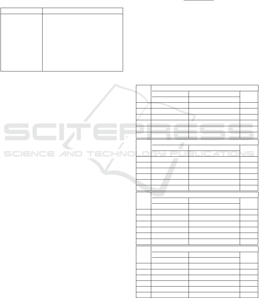
The obtained results are shown in Table 3. For each

instance, we report the average value of the global ob-

jective function obtained by running the 10 instances

for all of the four classes of tests, the elapsed time

(T(s)), the percentage of instances for which the pro-

posed CP ﬁnd the optimal solution and the RPD values.

Table 3: The results of the proposed CP model and the ones

of the MILP model on small instances.

SAI/LC

MILP CP

RPD

MILP

T(s) f

T(s) Best

9 423.20 3.39 435.35 2.02 90% 2.87%

10 402.75 2.87 410.90 2.18 80% 2.02%

11 439.85 12.39 445.65 2.18 90% 1.32%

12 503.20 197.73 508.40 2.80 90% 1.03%

13 416.75 553.67 427.30 2.79 90% 2.53%

AVG 88% 1.95%

SAI/HC

MILP CP

RPD

MILP

T(s) f

T(s) Best

9 135.05 3.34 141.25 2.14 90% 4.59%

10 147.55 3.37 155.50 2.15 70% 5.39%

11 174.85 5.98 179.15 2.57 90% 2.46%

12 216.00 18.15 219.85 3.38 80% 1.67%

13 183.45 84.56 183.45 2.37 100% 0%

AVG 86% 2.82%

LAI/LC

MILP CP

RPD

MILP

T(s) f

T(s) Best

9 304.50 10.02 304.50 2.61 100% 0%

10 284.80 17.95 289.45 2.52 70% 1.63%

11 355.95 61.10 362.05 3.17 80% 1.71%

12 366.85 553.67 385.30 4.51 60% 5.03%

13 348.55 634.32 353.45 3.88 50% 1.40%

AVG 72% 2.44%

LAI/HC

MILP CP

RPD

MILP

T(s) f

T(s) Best

9 106.80 3.93 106.80 2.08 100% 0%

10 121.65 3.26 122.10 2.57 90% 0.37%

11 147.35 7.82 151.25 2.65 70% 2.65%

12 176.40 18.56 182.60 3.15 60% 3.51%

13 172.40 159.80 172.40 2.83 100% 0%

AVG 70% 2.17%

The obtained results show that for all the tested in-

stances, the RPD does not exceed 5.40. We can even re-

A Constraint Programming Model for the Scheduling Problem with Flexible Maintenance under Human Resource Constraints

199

mark that the CP model ﬁnd the best solution in 100%

for four cases of the tests that are respectively Bench-

mark 9 (LAI/LC and LAI/HC classes) and Benchmark

13 (SAI/HC and LAI/HC classes). In average, the

RPD of each class of tests varies between 1.85 and

2.82. Furthermore, the best solution is found in more

than 80% when the intervals are strict and more than

70% when the intervals are large.

According to elapsed times, the CP model improves

the performance of the MILP model, especially on in-

stances where the size is between 11 and 13. We can

see that CP model spent between 2 s and 5 s to ﬁnd

the solution for all of the classes and all benchmarks.

It outperforms drastically the MILP model. However,

the MILP spent a considerable time to ﬁnd the optimal

solution for the benchmarks having a size ranking from

11 to 13, in comparison to CP model.

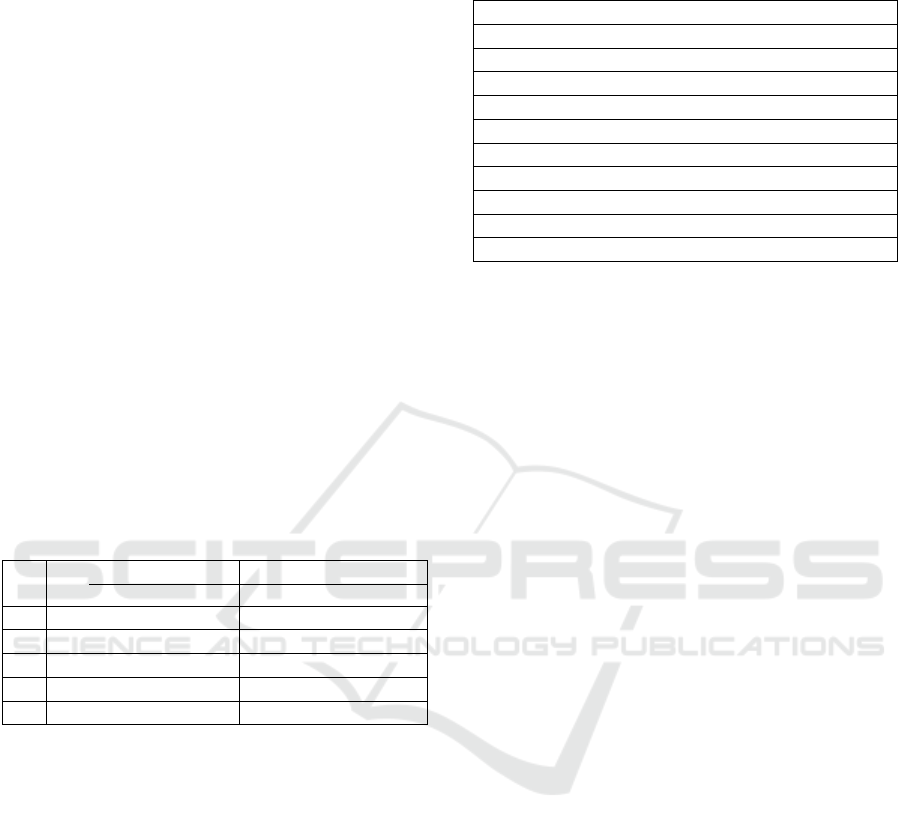
Another point to address, is the scalability of the

models. That is the number of variables (NV) and con-

straints (NC) involved in both models to encode each

instance. We present in Table 4 the average of these

data for each benchmark. For more analysis precision,

we present in Table 5 for the CP model, the number of

variables and constraints for all of the ten instances of

Benchmark 9.

Table 4: The number of variables and constraints of both

the CP and MILP models on small instances.

MILP CP

NV NC NV NC

9 180 151 19 17

10 186 171 20 16

11 239 215 22 18

12 272 252 25 21

13 255 269 24 18

We remark from Table 4 that both the number of

variables and constraints of the MILP are larger than

the ones of the CP model. This reason contributes in

the sense of obtaining elapsed times for the CP model

lower than those of the MILP models. We recall that

within a time limit set at one hour, the MILP model

could not resolve instances with a size greater than 13.

The difference in number of variables (NV) and num-

ber of constraints (NC) of the MILP model is of the or-

der of nine times the measurements in number of vari-

ables and constraints of the CP model. In addition, this

gap tends to increase when the number of variables in-

creases, thus making the CP model more advantageous

for solving large instances.

Table 5: The number of variables and constraints of the CP

model of Benchmark 9.

Instance VN CN

1 22 21

2 18 15

3 22 21

4 22 21

5 14 9

6 22 21

7 18 15

8 22 21

9 22 21

10 14 9

Now, if we are interested in the particular case of

Benchmark 9 of the CP model given in Table 5, we can

notice that the number of variables varies between 14

and 22 and the number of constraints varies between

9 and 21. Generally the number of the variables and

constraints of an instance of this problem depend on

its number of production tasks and the number of its

maintenance tasks. As the number of production tasks

is ﬁxed at 9 for the ten instances of Benchmark 9, we

understand that the variation of the number of variables

NV and that one of the constraints NC comes from the

fact that the number of maintenance activities changes.

4.2 Results of the CP Model on Large

Size Instances

As we mentioned previously, we extended the exper-

iments to larger size instances. It should be noted

that the free version of IBM Ilog Cplex reaches its

calculation limits when the size of the benchmark is

equals to 60 jobs. Indeed, Ilog CP Optimizer Commu-

nity Edition solves problems with search spaces up to

1000

. We consider here the benchmarks having the size

N ∈ {15,18,20, 40,60}. We generated ten instances for

each of the four classes of each benchmark. In total, we

experimented 5X10X4=200 tests. First, we considered

Benchmark 20 that we experimented in order to ﬁx the

execution time limits to one hour. We remarked that for

the majority of the generated instances (80% of the in-

stances) for this benchmark, the best solutions is found

in less than one hour. Then for the rest of instances, we

ﬁxed the time limit to one hour.

The obtained results are shown in Table 6. For each

benchmark and class of tests, we give the average val-

ues of all of the production, the maintenance, the global

objective functions and the elapsed times (T(s)) spent

to solve the considered instance.

First of all, we can see in Table 6 that with the CP

model we manage to solve instances of this problem

containing up to 60 production tasks in one hour of

elapsed time while the MILP model fails to resolve in-

stances of this problem having more than 13 production

ICAART 2022 - 14th International Conference on Agents and Artiﬁcial Intelligence

200

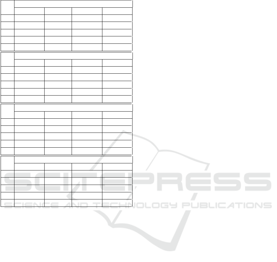
Table 6: The CP results for the large size problems.

SAI/LC

f T (s)

15 2316.90 269.00 1292.95 16.67

18 2919.3 347.8 1633.55 304.86

20 4275.80 361.70 2318.75 3309.60

40 16205.50 755.90 8490.75 3600

60 27275.60 1173.10 14224.35 3600

SAI/HC

f T (s)

15 683.50 44.90 364.20 10.80

18 784.3 72.3 428.3 18.292

20 1246.40 109.60 678.00 445.05

40 5420.20 214.30 2816.75 3600

60 7353.70 363.20 3873.30 3600

LAI/LC

f T (s)

15 1629 146 887.5 67.086

18 2644.7 235.3 1439 1048.638

20 3591.80 282.90 1936.35 2741.16

40 13766.20 539.70 7155.40 3600

60 25020.50 852.30 12936.40 3600

LAI/HC

f T (s)

15 591.4 26.50 308.95 13.675

18 714.4 27.4 370.9 16.61

20 1061.50 50.20 555.85 577.24

40 4943.20 117.00 2542.25 3600

60 6947.00 191.30 3569.15 3600

jobs under the same elapsed time condition.

We can note that the order of magnitude of the

elapsed time changes from a few seconds for the in-

stances having 15 production tasks to a few minutes for

the instances having 18 production tasks then changes

approximately to one hour time for the instances hav-

ing more than 20 production tasks. This proves the

high impact of availability constraints even when the

number of production tasks does not increase signiﬁ-

cantly. But the tendency remains that the complexity

varies exponentially depending on the number of pro-

duction tasks that represent the size of the problem.

We can see that, for all benchmarks, the quality

of the three objective functions f

, f

, and f is better

when considering human resource with high compe-

tence (HC) for both classes of instances SAI and LAI.

More precisely, we got the rank LAI/HC, SAI/HC,

LAI/LC and SAI/LC for the different classes. The

main reason of this result is due to the fact that a main-

tenance operation executed by a human resource with

a high competence and large availability intervals has

more possible insertion sites and consequently it leads

to more opportunities to optimize the objective func-

tion. Indeed, with a high competence, the mainte-

nance duration decreases and could be inserted inside

its tolerance interval since the human resource has large

availability intervals.

In summary, we can say that the CP model repre-

sents a considerable improvement for the MILP model.

We recall that the CP model ﬁnds the optimal solu-

tion in almost 80% of cases and when the latter is not

reached it returns a good solution very close to the op-

timal. This model then represents a very good compro-

mise between the exact MILP model and the non-exact

methods called metaheuristics.

5 CONCLUSION

In this paper, we deal with the scheduling problem of

production and maintenance activities that considers

the competence and availability human resource con-

straints.

The main contribution of this paper is the introduc-

tion of a CP model to formulate the studied schedul-

ing problem. This CP model had been implemented

in OPL language and presents a good alternative to the

MILP modeling proposed in (Touat et al., 2021).

To validate our CP model, we used it to express

several instances of the problem that we solved with

the IBM Ilog Cplex software engine and compared our

approach to the MILP model (Touat et al., 2021) on

small instances. The obtained results show that the

proposed CP model is powerful and outperforms the

MILP model. Also, it is a good compromise between

exact methods like the the MILP approach and meta-

heuristics, since it usually succeeds to ﬁnd the optimal

solutions in approximately 79% of the checked small

instances in a very low elapsed time.

Further, the CP model was used to represent and

solve relatively large instances of the studied problem.

We were able to solve instances with up to 60 produc-

tion tasks in one hour of elapsed time while the MILP

model cannot resolve instances of more than 13 pro-

duction tasks in one hour of lab time.

For future work and perspectives, we ﬁrst plan to

study a multi-objective version of the problem and

compare it to the version introduced in this work, then

we want to generalize our study for versions of the

problem with several machines.

REFERENCES

Chen, J.-S. (2008). Scheduling of nonresumable jobs and

ﬂexible maintenance activities on a single machine to

minimize makespan. The International Journal of Ad-

vanced Manufacturing Technology, 190:90–102.

Cui, W.-W. and Lu, Z. (2014). Integrated production

scheduling and periodic maintenances on a single ma-

chine with release dates. IEEE International Confer-

A Constraint Programming Model for the Scheduling Problem with Flexible Maintenance under Human Resource Constraints

201

ence on Automation Science and Engineering (CASE),

197:Taipei, Taiwan.

Graham, R.-L., Lawler, E.-L., Lenstra, J.-K., and Kan, A.-

R. (1979). Optimization and approximation in deter-

ministic sequencing and scheduling: a survey. Annals

of discrete mathematics, 5:287–326.

Ham, A. (2020). ransfer-robot task scheduling in job shop.

International Journal of Production Research, DOI:

10.1080/00207543.2019.1709671.

Hauder, V.-A., Beham, A., Raggl, S., Parraghb, S.-N., and

Affenzeller, M. (2020). Resource-constrained multi-

project scheduling with activity and time fexibility.

IComputers and Industrial Engineering.

J. Kinable, W.-J. v. H. and Smith, S.-F. (2021). Snow

plow route optimization: A constraint programming

approach. IISE Transactions, 53:6:685–703.

Kan, A.-R. (1976). Machine scheduling problems: classiﬁ-

cation, complexity and computations. Springer.

Kress, D. and M

uller, D. (2019). Shop scheduling problem

with machine operator constraints. IFAC PapersOn-

Line, pages 94–99.

Laborie, P. (2009). Ibm ilog cp optimizer for de-

tailed scheduling illustrated on three prob-

lems. Lecture Notes in Computer Science,

https://doi.org/10.1007/978-3-642-01929-6-12.

Laborie, P., Rogerie, J., Shaw, P., and Vilim, P. (2018).

Ibm ilog cp optimizer for scheduling: 20+ years of

scheduling with constraints at ibm/ilog. Constraints,

https://doi.org/10.1007/s10601-018-9281-x.

Lee, C.-Y. and Liman, S.-D. (1992). Single machine ﬂow-

time scheduling with scheduled maintenance. Acta In-

formatica, 29:375–382.

Liu, M., Wang, S., Chu, C., and Chu, F. (2015). An im-

proved exact algorithm for single-machine scheduling

to minimise the number of tardy jobs with periodic

maintenance. International Journal of Production Re-

search, DOI:10.1080/00207543.2015.1108535.

Low, C., Ji, M., Hsu, C.-J., and Su, C.-T. (2010). Mini-

mizing the makespan in a single machine scheduling

problems with ﬂexible and periodic maintenance. Ap-

plied Mathematical Modelling, 34:334–342.

Lunardi, W.-T., Birgin, E.-G., Laborie, P., Ronconi,

D.-P., and Voos, H. (2020). Mixed integer lin-

ear programming and constraint programming mod-

els for the online printing shop scheduling prob-

lem. Optimization and Control (math.OC), DOI:

10.1016/j.cor.2020.105020.

Luo, A., Cheng, T.-C.-E., and Ji, M. (2015). Single-

machine scheduling with a variable maintenance ac-

tivity wenchang. Computers and Industrial Engineer-

ing, 79:168–174.

Mashkani, O. and Moslehi, G. (2016). Minimising the total

completion time in a single machine scheduling prob-

lem under bimodal ﬂexible periodic availability con-

straints. International Journal of Computer Integrated

Manufacturing, 29:323–341.

Mokhtarzadeh, M., Tavakkoli-Moghaddam, R., Vahedi-

Nouri, B., and Farsi, A. (2020). Scheduling of

human-robot collaboration in assembly of printed cir-

cuit boards: a constraint programming approach. In-

ternational Journal of Computer Integrated Manufac-

turing, DOI: 10.1080/0951192X.2020.1736713.

Ornek, M.-A., Ozturk, C., and Sugut, I. (2020). Inte-

ger and constraint programming model formulations

for ﬂight-gate assignment problem. Operational Re-

search, https://doi.org/10.1007/s12351-020-00563-9.

Polo-Mej

ıa, O., Artigues, C., Lopez, P., and Basini, V.

(2019). Mixed-integer/linear and constraint program-

ming approaches for activity scheduling in a nuclear

research facility. International Journal of Production

Research, DOI:10.1080/00207543.2019.1693654.

Qin, T., Du, Y., Chen, J.-H., and Sha, M. (2020). Combining

mixed integer programming and constraint program-

ming to solve the integrate d scheduling problem of

container handling operations of a single vessel. Euro-

pean Journal of Operational Research, 285:884–901.

Touat, M., Benbouzid, F., and Benhamou, B. (2021). Exact

and metaheuristic approaches for the single-machine

scheduling problem with ﬂexible maintenance under

human resource constraints. International Journal of

Manufacturing Research.

Touat, M., Bouzidi-Hassini, S., Benbouzid-Sitayeb, F., and

Benhamou, B. (2017). A hybridization of genetic

algorithms and fuzzy logic for the single-machine

scheduling with ﬂexible maintenance problem under

human resource constraints. Applied Soft Computing,

59:556–573.

Touat, M., Tayeb, F. B.-S., and Benhamou, B. (2018).

An effective heuristic for the single-machine schedul-

ing problem with ﬂexible maintenance under human

resource constraints. Procedia Computer Science,

126:1395–1404.

Yang, S.-L., Maa, Y., Xu, D.-L., and Yang, J.-B. (2011).

Minimizing total completion time on a single machine

with a ﬂexible maintenance activity. Computers and

Operations Research, 38:755–770.

Yazdani, M., Khalili, S.-M., Babagolzadeh, M., and Jolai,

F. (2017). A single-machine scheduling problem with

multiple unavailability constraints: A mathematical

model and an enhanced variable neighborhood search

approach. Journal of Computational Design and En-

gineering, 4:46–59.

Zammori, F., Braglia, M., and Castellano, D. (2014). Har-

mony search algorithm for single-machine scheduling

problem with planned maintenance. Computers I&

Industrial Engineering, 76:333–346.

ICAART 2022 - 14th International Conference on Agents and Artiﬁcial Intelligence

202