Solver-based Approaches for Robust Multi-index Selection Problems

with Stochastic Workloads and Reconﬁguration Costs

Marcel Weisgut, Leonardo H

ubscher, Oliver Nordemann and Rainer Schlosser

Hasso Plattner Institute, University of Potsdam, Potsdam, Germany

Keywords:

Resource Allocation Problems, Stochastic Workloads, Index Selection, Robustness, Linear Programming.

Abstract:

Fast processing of database queries is a primary goal of database systems. Indexes are a crucial means for

the physical design to reduce the execution times of database queries signiﬁcantly. Therefore, it is of great

interest to determine an efﬁcient selection of indexes for a database management system (DBMS). However, as

indexes cause additional memory consumption and the storage capacity of databases is limited, index selection

problems are highly challenging. In this paper, we consider a basic index selection problem and address

additional features, such as (i) multiple potential workloads, (ii) different risk-averse objectives, (iii) multi-

index conﬁgurations, and (iv) reconﬁguration costs. For the different problem extensions, we propose speciﬁc

model formulations, which can be solved efﬁciently using solver-based solution techniques. The applicability

of our concepts is demonstrated using reproducible synthetic datasets.

1 INTRODUCTION

In this paper, we consider resource allocation prob-

lems in database systems using means of quantitative

methods and operations research. Speciﬁcally, to be

able to run database workloads efﬁciently, we opti-

mize whether and where to store certain auxiliary data

structures such as indexes.

1.1 Background

Indexes in a relational database system are auxiliary

data structures used to reduce the execution time re-

quired for generating the result of a database query.

The shorter the execution time of a workload’s query

set, the more queries can be executed per time unit.

Consequently, reducing query execution times implic-

itly increases the throughput of the database. Indexes

are data structures that have to be stored in addition to

the stored data of a database itself, which leads to ad-

ditional memory consumption and increases the over-

all memory footprint of the database. Memory ca-

pacity is limited and, therefore, a valuable resource.

For this reason, it is important to take the memory

consumption into account for decision making about

which indexes to store in the system’s memory.

For a single database query, multiple indexes may

exist, each of which can improve the query execution

time differently. Table 1 shows an exemplary scenario

in which different combinations of indexes lead to dif-

ferent execution times of a single hypothetical exam-

ple query. The ﬁrst combination without any index

leads to the longest execution time of the query with

500 milliseconds. The best execution time of 300 mil-

liseconds can be achieved by using both index 1 and

index 2. However, the best performing combination

regarding the execution time also involves the largest

memory footprint. The second-best solution from an

execution time perspective results in an index mem-

ory consumption of only 40% of the optimal solution

and is only about 17% slower. This simple example

illustrates the need to consider the index memory con-

sumption for selecting which indexes should be used.

In real-world database scenarios, a DBMS pro-

cesses more than only a single query. Instead, a set of

queries is executed on a database with a certain fre-

quency in a speciﬁc time frame for each query. The

Table 1: Sample index combinations with their memory

consumption and the resulting execution times of a hypo-

thetical query.

Usage of

index 1

Usage of

index 2

Total memory

footprint

Query

execution time

false false 0 MB 500 ms

true false 100 MB 350 ms

false true 150 MB 400 ms

true true 250 MB 300 ms

Weisgut, M., Hübscher, L., Nordemann, O. and Schlosser, R.

Solver-based Approaches for Robust Multi-index Selection Problems with Stochastic Workloads and Reconﬁguration Costs.

DOI: 10.5220/0010800600003117

In Proceedings of the 11th International Conference on Operations Research and Enterprise Systems (ICORES 2022), pages 28-39

ISBN: 978-989-758-548-7; ISSN: 2184-4372

set of queries with their frequencies is referred to as

workload. Executing a workload using a selection

of indexes has a certain performance. This perfor-

mance is characterized by the total execution time of

the workload and the selected indexes’ memory con-

sumption. The workload execution time should be as

low as possible, and the index memory consumption

must not exceed a speciﬁc memory budget.

An additional challenge of selecting the set of in-

dexes that shall be present and used by queries is in-

dex interaction. ”Informally, an index a interacts with

an index b if the beneﬁt of a is affected by the pres-

ence of b and vice-versa.” (Schnaitter et al., 2009)

For example, assume a particular index i for a subset

S of the overall workload may provide the best per-

formance improvement for each query in that subset.

There is also no other index that has a better accu-

mulated performance improvement. Suppose i now

has such a high memory consumption that the avail-

able index memory budget is completely spent. In

that case, no other index can be created. Therefore,

only queries of the subset S are improved by index i.

Another index selection might be worse for the work-

load subset S but better for the overall workload. Con-

sequently, a (greedily chosen) single index whose ac-

cumulated performance improvement is the highest is

not necessarily in the set of indexes that provides the

best performance improvement for the total workload.

1.2 Contribution

In this work, we present solver-based approaches to

address speciﬁc challenges of index selection that oc-

cur in practice. Besides one basic problem, solution

concepts for four extended problem versions are pro-

posed. Our contributions are the following:

• We study solver-based approaches for single- and

multi-index selection problems.

• We use a ﬂexible chunk-based heuristic approach

to attack larger problems.

• We consider extensions with multiple stochastic

workload scenarios and reconﬁguration costs.

• We derive risk-aware index selections using worst

case and variance-based objectives.

• We use reproducible examples to test our ap-

proaches, which can be easily combined.

The remainder of this work is structured as fol-

lows. Section 2 summarizes related work. In Sec-

tion 3, the various index selection problems are for-

mulated, and their solutions are presented. Section 4

then brieﬂy describes how the models were imple-

mented. An evaluation of the developed models is

given in Section 5. In Section 6, we discuss future

work. Finally, Section 7 concludes this work.

2 RELATED WORK

Index recommendation and automated selection have

been in the focus of database research for many

years and are still important today, particularly in the

rise of self-optimizing databases (Pavlo et al., 2017;

Kossmann and Schlosser, 2020). Next, we give an

overview index selection algorithms.

An overview of the historic development as well

as an evaluation of index selection algorithms is sum-

marized by Kossmann et al. (Kossmann et al., 2020).

Current state-of-the-art index selection algorithms

are, e.g., AutoAdmin (Chaudhuri and Narasayya,

1997), DB2Advis (Valentin et al., 2000), CoPhy

(Dash et al., 2011), DTA (Chaudhuri and Narasayya,

2020), and Extend (Schlosser et al., 2019). All those

selection approaches focus on deterministic work-

loads. Risk-aversion in case of multiple potential

workloads is not supported. As typically iterated or

recursive methods are used, it is not straightforward

how they have to be amended to address the exten-

sions considered in this paper, such as multiple work-

loads, risk-aversion, or transition costs.

Early approaches tried to derive optimal index

conﬁgurations by evaluating attribute access statis-

tics (Finkelstein et al., 1988). Newer index selec-

tion approaches are mostly coupled with the query

optimizer of the database system (Kossmann et al.,

2020). By doing so, the costs models of the index

selection algorithm and the optimizer are the same.

As a result, the beneﬁt of considered indexes can

be estimated consistently (Chaudhuri and Narasayya,

1997). As optimizer invocations are costly, especially

for complex queries, along with improved index se-

lection algorithms, techniques to reduce and speed up

optimizer calls have been developed (Chaudhuri and

Narasayya, 1997; Papadomanolakis et al., 2007; ?).

An increasing number of possible optimizer calls

for index selection algorithms opens the possibility

to investigate an increasing number of index can-

didates. Compared to greedy algorithms (Chaud-

huri and Narasayya, 1997; Valentin et al., 2000), ap-

proaches using mathematical optimization are able

to efﬁciently evaluate index combinations. In this

context, we perceive a shift away from greedy al-

gorithms (Chaudhuri and Narasayya, 1997; Valentin

et al., 2000) towards approaches using mathematical

optimization models and methods of operations re-

search, especially integer linear programming (ILP)

(Casey, 1972; Dash et al., 2011). A major challenge

Solver-based Approaches for Robust Multi-index Selection Problems with Stochastic Workloads and Reconﬁguration Costs

of these solver-based approaches is to deal with the in-

creasing complexity of integer programs. An obvious

solution is reducing the number of initially considered

index candidates, which may, however, reduce the so-

lution quality.

Alternatively, also machine learning-based ap-

proaches for index selection are an emerging research

direction. For example, deep reinforcement learning

(RL) have already been applied, cf., e.g., (Sharma

et al., 2018) or (Kossmann et al., 2022). Such ap-

proaches, however, require extensive training, and are

still limited with regard to large workloads or multi-

attribute indexes, and do not support risk-averse opti-

mization criteria.

3 SOLUTION APPROACH

In this section, a basic index selection problem and its

extensions are formulated, and the solutions for each

problem are presented. Section 3.1 describes a ba-

sic index selection problem, which is considered the

basic problem in this work. In addition to the prob-

lem’s description, we formulate an integer linear pro-

gramming model, which can solve this problem. Sec-

tions 3.2, 3.3, 3.4, and 3.5 each describe an extension

of the basic problem and explain which adjustments

can be made to the solution of the basic problem to

solve the specialized problems. Finally, Section 3.6

describes the problem in which all advanced problems

were combined.

3.1 Basic Problem

In this subsection, we ﬁrst describe a basic version

of the index selection problem, which resembles typ-

ical properties. The basic index selection problem is

about ﬁnding a subset of a given set of index (multi-

attribute) candidates used by a hypothetical database

to minimize the total execution time of a given work-

load. The given workload consists of a set of queries

and a frequency for each query. A query can use

no index or exactly one index for support. Differ-

ent indexes induce different improvements for a sin-

gle query. As a result, the execution time of a query

highly depends on the used index. A query has the

longest execution time if no index is used. For each

query, it has to be decided whether and which index

is to be used. Only if at least one query uses an in-

dex, the index can belong to the set of selected in-

dexes. Each index involves a certain amount of mem-

ory consumption. The total memory consumption of

the selected indexes must not exceed a predeﬁned in-

dex memory budget.

Table 2: Basic parameters and decision variables.

Designation Type Description

I parameter number of indexes

Q parameter number of queries

M parameter index memory budget

q,i

parameter

execution time of query

q = 1, ..., Q using index

i = 0, ..., I; i = 0

indicates that no index

is used by query q

parameter

memory consumption of

index i = 1, ..., I

parameter

frequency of query

q = 1, ..., Q

q,i

decision

variable

binary variable whether

index i = 0, ..., I is used

for query q = 1, ..., Q;

i = 0 indicates that no

index is used by query q

decision

variable

binary variable whether

index i = 1, ..., I is used

for at least one query

Table 2 shows the formal representation of the

given parameters and the decision variables of our

model. The binary variable u

q,i

∈ {0, 1} is used to

control whether an index i is used for query q. Vari-

able v

∈ {0, 1} indicates whether index i is selected

overall. It is used to calculate the overall memory con-

sumption of selected indexes. Similar to the work of

Schlosser and Halfpap (Schlosser and Halfpap, 2020),

the considered standard basic index selection problem

can be formulated as an integer LP model:

minimize

q,i

∈{0,1}

I+Q×(I+1)

∑

q=1,...,Q

i=0,...,I

q,i

·t

q,i

· f

(1)

s.t.

∑

i=1,...,I

· m

≤ M (2)

∑

i=0,...,I

q,i

= 1, q = 1, ..., Q (3)

∑

q=1,...,Q

q,i

≥ v

, i = 1, ..., I (4)

∑

q=1,...,Q

q,i

≤ v

, i = 1, ..., I (5)

The objective (1) minimizes the execution time of

the overall workload taking into account the index us-

age for queries, the index-dependent execution times,

ICORES 2022 - 11th International Conference on Operations Research and Enterprise Systems

and the frequency of queries. The constraint (2) en-

sures that the selected indexes do not exceed the given

memory budget M. Constraint (3) ensures that a max-

imum of one index is used for a single query. Here, a

unique option has to be chosen including the no index

option. Thus, if u

q,i

with i = 0 is true, no index is used

for query q. The constraints (4) and (5) are required to

connect u

q,i

with v

. If no query uses a speciﬁc index

i, constraint (4) ensures that v

is equal to 0 for that

index. If at least one query uses index i, constraint (5)

ensures that v

is equal to 1 for that index.

3.2 Chunking

The number of possible solutions of the index selec-

tion problem grows exponentially with the number of

index candidates. Databases for modern enterprise

applications consist of hundreds of tables and thou-

sands of columns. This leads to long execution times

to ﬁnd the optimal solution of the increasing prob-

lem. In this extension, the set of possible indexes is

split into chunks of indexes. The index selection prob-

lem will then be solved via (1) - (5) only with the re-

duced set of indexes for each chunk, and the indexes

of the optimal solution will be returned. After solving

the problem for each chunk, the best indexes of each

chunk will get on. In the second round, the reduced

number of remaining indexes will be used for a ﬁnal

selection using again (1) - (5).

The approach allows an effective problem decom-

position and accounts for index interaction. Naturally,

chunking remains a heuristic approach an does not

guarantee an optimal solution, but the main advantage

is to avoid large problems. Of course chunks should

not be chosen too small as splitting the global prob-

lem into too many local problems can also add over-

head (see the evaluations presented in Section 5.4).

An other advantage is that, in the ﬁrst round, all the

chunks could be solved in parallel. With this, the

overall execution time could be reduced even further.

3.3 Multi-index Conﬁguration

Our basic problem introduced in Section 3.1 could not

handle the interaction of indexes as described in the

introduction: One query could be accelerated by more

than one index and the performance gain of an index

could be affected by other indexes. We tackle this part

of the index selection problem by adding one level of

indirection called index conﬁgurations.

An index conﬁguration maps to a set of indexes.

Assuming the index selection problem has ten in-

dexes, then the ﬁrst conﬁguration (conﬁguration 0)

means that no index is used for this query. The next

ten possible conﬁgurations point to the respective in-

dexes, e.g., conﬁguration 1 points to index 1, conﬁg-

uration 2 points to index 2, conﬁguration 10 points to

index 10. The subsequent conﬁgurations map to sets

containing combinations of two indexes. Database

queries could be accelerated by more than two in-

dexes, but we simpliﬁed the conﬁgurations in our im-

plementation so that they can consist of a maximum

of two different indexes. We use a binary parame-

ter d

c,i

indicating whether conﬁguration c contains the

index i. c = 0, ..., C and i = 0, ..., I with C being the

number of index conﬁgurations and I being the num-

ber of indexes. Furthermore, we assume that ten per-

cent of all possible index combinations will interact

in conﬁgurations. Our approach to index selection

works with conﬁgurations in the same way as with

indexes, cf. (1) - (5). The constraints (3) - (5) of the

basic problem, cf. Section 3.1, are adapted in the fol-

lowing way for multi-index conﬁgurations:

∑

c=0,...,C

q,c

= 1, q = 1, ..., Q (6)

∑

q=1,...,Q

q,c

· d

c,i

≥ v

c = 1, ..., C

i = 1, ..., I

(7)

∑

q=1,...,Q

q,c

· d

c,i

≤ v

c = 1, ..., C

i = 1, ..., I

(8)

Again, the binary variable u

q,c

is used to control if

conﬁguration c is used for query q and C is the num-

ber of index conﬁgurations. Similar to the basic ap-

proach, c = 0 represents a conﬁguration that contains

no index. Constraint (6) ensures that one single query

uses exactly one conﬁguration option instead of one

index. In constraint (7) - (8), the parameter d

c,i

is in-

cluded to activate indexes of used conﬁgurations.

3.4 Stochastic Workloads

Until now, we considered a single given workload

only. However, in the context of enterprise applica-

tions, we could imagine that each day of the week has

a different workload. For example, the workloads on

the weekend could contain fewer requests compared

to a workload during the week. In this section, we

propose an approach that can take multiple workloads

into account. The solution seeks to provide a robust

index selection, where robust means that the perfor-

mance is good no matter which workload may occur.

First, the expected total workload cost T across all

workloads is being calculated as

T =

∑

w=1,...,W

∑

=1,...,W

(9)

Solver-based Approaches for Robust Multi-index Selection Problems with Stochastic Workloads and Reconﬁguration Costs

Figure 1: Exemplary costs for each workload when mini-

mizing the global costs (lower is better).

where W is the number of different workloads. To

describe workload probabilities, we use the intensities

, w = 1, ..., W . Further, the execution time g

of a

workload w is determined by (10), with f

w,q

being the

frequency of query q in workload w, w = 1, ..., W , i.e.,

∑

q=1,...,Q, c=1,...,C

q,c

·t

q,c

· f

w,q

(10)

The information whether a conﬁguration c is be-

ing used for a query q of a workload w is shared be-

tween the workloads, leaving it to the solver to mini-

mize the total costs across all workloads.

Figure 1 shows exemplary total workload costs

when minimizing the global execution time. It can

be seen that the actual costs of each workload differ a

lot, leading to poor performances for W 1 and W 3 in

favor of W 2 and W 4. We use two different approaches

to make the index selection more robust.

The ﬁrst one includes the worst-case performance

by punishing the total costs with the maximum work-

load costs as additional costs. The maximum work-

load costs L (modelled as a continuous variable) are

determined by the constraint:

L ≥ g

∀w = 1, ..., W (11)

The following (mixed) ILP, cp. (1) - (5), now in-

cludes this maximum workload cost (L) in the objec-

tive using the penalty factor a ≥ 0, cf. (9) - (10):

minimize

q,i

∈{0,1}

I+Q×(I+1)

, L∈R

T + a · L (12)

Figure 2 illustrates a typical solution leading to

better worst-case cost, cp. Figure 1. However, the

costs of W 2 and W 3 increased, leaving also a bigger

gap between W 4 and the rest.

To obtain robust performances, the second ap-

proach uses the variance V , cf. (9) - (10),

V =

∑

w=1,...,W

− T )

∑

=1,...,W

(13)

Figure 2: Exemplary workload costs with increased robust-

ness by optimizing the worst-case costs.

Figure 3: Exemplary workload costs with increased robust-

ness by using the mean-variance criterion.

of the workload costs as a penalty to minimize the

scenarios’ cost differences. Now, the factor b and the

term b ·V is used in the objective, cp. (12) - (13),

minimize

q,i

∈{0,1}

I+Q×(I+1)

T + b ·V (14)

Remark that the problem, cf. (14), becomes a bi-

nary quadratic programming (BQP) problem by us-

ing the variance V in the penalty term. Using the

mean-variance criterion (14) typically leads to results

illustrated in Figure 3. Typically, all costs are now

within a similar range. However, in comparison to the

previous ﬁgures, not only have been W 1, W 2 and W 3

brought into a plannable range, but also W4. The to-

tal costs of W 4 may not be reduced, which makes the

result indeed more robust but less effective in the end.

A third option to resolve this issue would be to use

the semi-variance instead of V . Similar to the vari-

ance, the semi-variance can be used to penalize only

those workloads whose costs are higher than the mean

cost of all workloads, i.e., workloads with lower costs

would not increase the applied penalty.

Finally, the proposed risk-averse approaches

enables us to use potential workloads (e.g., observed

in the past) to optimize index selections for stochastic

future scenarios under risk considerations.

ICORES 2022 - 11th International Conference on Operations Research and Enterprise Systems

Table 3: Transition cost calculation example.

Index v

∗

RM + MK

# mk

1 50 10 1 1 0 (keep)

2 20 5 0 1 20 (create)

3 100 30 1 0 30 (remove)

4 10 1 0 0 0 (skip)

Total transition costs 50

3.5 Transition Costs

In the previous subsections, we showed how to deal

with different workloads, e.g., on consecutive days.

In this problem extension, we consider the costs of

a transition from one index conﬁguration to another.

We assume that the database removes indexes that are

no longer used and loads indexes that are to be used

into the memory. Typically, the database would need

to do some I/O operations, which are time expensive

and generate additional costs. We model such cre-

ation and removal costs in our ﬁnal extension to re-

duce such transition costs.

To adapt the index conﬁgurations, the algorithm

identiﬁes the differences between the previous con-

ﬁguration (now characterized by parameters v

∗

) and

a new target conﬁguration governed by the variables

. For each removal at index i, the algorithm looks

up the removal costs rm

for index i and adds them to

the total removal costs RM. Analogous, the algorithm

proceeds to calculate the total creation costs MK us-

ing the creation costs mk

of the index i. The sum

of the removal costs and creation costs is then being

added to any of the previous objectives, which allows

to avoid high transition costs. The costs can be mod-

elled linearly:

RM =

∑

i=1,...,I

∗

· (1 − v

) · rm

(15)

MK =

∑

i=1,...,I

· (1 − v

∗

) · mk

(16)

Table 3 describes an explanatory calculation of the

transition costs between two index selections. The

previous selection (v

∗

) uses the indexes 1 and 3. The

new selection (v) uses index 1 and 2. The resulting

transition costs are 50.

3.6 Combined Problem

All extensions described in the previous subsections

were developed on top of the basic approach. To

show the encapsulation of all extensions, we also im-

plemented a solution that integrates all extensions in

an all-in-one solution. In most of the cases, this

is straightforward as all key concepts are indepen-

dent from each other and no coupling is involved.

However, when combining multiple components the

model’s complexity increases. Hence, we recommend

to use only those features that are really needed in spe-

ciﬁc applications.

4 IMPLEMENTATION

To evaluate the described approaches, we imple-

mented our different models using AMPL

, which is

a modeling language tailored for working with op-

timization problems (Fourer et al., 2003). The syn-

tax of AMPL is quite close to the algebraic one and

should be easy to read and understand, even for the

readers, who have never seen AMPL syntax before.

AMPL itself translates the given syntax into a format

solvers can understand.

The solver is a separate program that needs to be

speciﬁed by the developer. The approach is based on

linear/quadratic programming using integer numbers.

Both solvers, CPLEX

and Gurobi

, are suited to

solve the index selection task. A ﬁrst test showed that

Gurobi is faster than CPLEX in most cases, which is

the reason why we used Gurobi.

The .run-ﬁle contains information about the se-

lected solver and loads the speciﬁed model and data

speciﬁcations. After a given problem was solved, the

solution is displayed. The .mod-ﬁle contains the de-

scription of the mathematical model, such as parame-

ters, constraints, and objectives used. The input data,

which is required for solving a certain problem, is

speciﬁed in the .dat-ﬁle. All code ﬁles are available

at GitHub

. Our implementation in AMPL allows the

reader to evaluate the different approaches and to re-

produce its results, see Section 5.

5 EVALUATION

In this section, we evaluate our approach. The con-

sidered setup and the input data are described in

Section 5.1 and Section 5.2, respectively. In Sec-

tion 5.3, we reﬂect on the scalability of the basic ap-

proach. Then, in Section 5.4, we investigate when in-

dex chunking is beneﬁcial for the performance com-

pared to the basic approach and reﬂect on the cost

https://ampl.com/

https://www.ibm.com/de-de/analytics/cplex-optimizer

https://www.gurobi.com/de/

https://github.com/mweisgut/DDDM-index-selection

Solver-based Approaches for Robust Multi-index Selection Problems with Stochastic Workloads and Reconﬁguration Costs

trade-off that the heuristic entails. Afterward, in Sec-

tion 5.5, we determine the computational overhead of

the multi-index extension. Lastly, in Section 5.6, we

take a more in-depth look into the stochastic work-

load extension, evaluating the impact of the different

robustness measures and the trend of costs depending

on the number of potential workloads.

5.1 Evaluation Setup

All performance measurements were performed on

the same machine, featuring an Intel i5 8th genera-

tion (4 cores) and 8GB memory storage. All mea-

surements were repeated three times. For each time

measurement, we used the AMPL build-in function

total solve time. It returns the user and system CPU

seconds used by all solve commands.

The ﬁnal value was determined by the mean of all

three measurement results. All non-related applica-

tions have been closed to reduce any side effects of

the operating system.

5.2 Datasets

The datasets that are being used for the evaluation are

being generated randomly, using multiple ﬁxed ran-

dom seeds. Each dataset is deﬁned by the number

of indexes, queries, and available memory budget.

The algorithm provided in the index-selection.data-

ﬁle then generates the execution time of each query,

depending on the utilized index. Firstly, the “original”

execution time for the query without using any in-

dex are chosen randomly within the interval [10;100].

Based on the drawn costs, the speedup for each in-

dex is calculated by choosing a random value between

the “original” costs and a 90% speedup. The memory

consumption of a query can be an integer between 1

and 20. The frequencies can be between 1 and 1 000.

The extensions that are applied on top of the ba-

sic approach introduce further variables that need to

be generated. For the stochastic workload extension,

we introduced a workload intensity, which gets drawn

randomly for each workload. This also applies to the

transition cost extension, where the creation costs and

removal costs are random. The multi-index conﬁgu-

rations package requires a more complex generation

process since each index conﬁguration should be a

unique set of indexes. The conﬁguration zero repre-

sents the option that no index is being used. The con-

ﬁgurations 1 to I point to their respective single index.

All other generated conﬁgurations consist of up to

two indexes, whereas the combinations are drawn ran-

domly. By using a second data structure, it is ensured

that no index combination is used multiple times. The

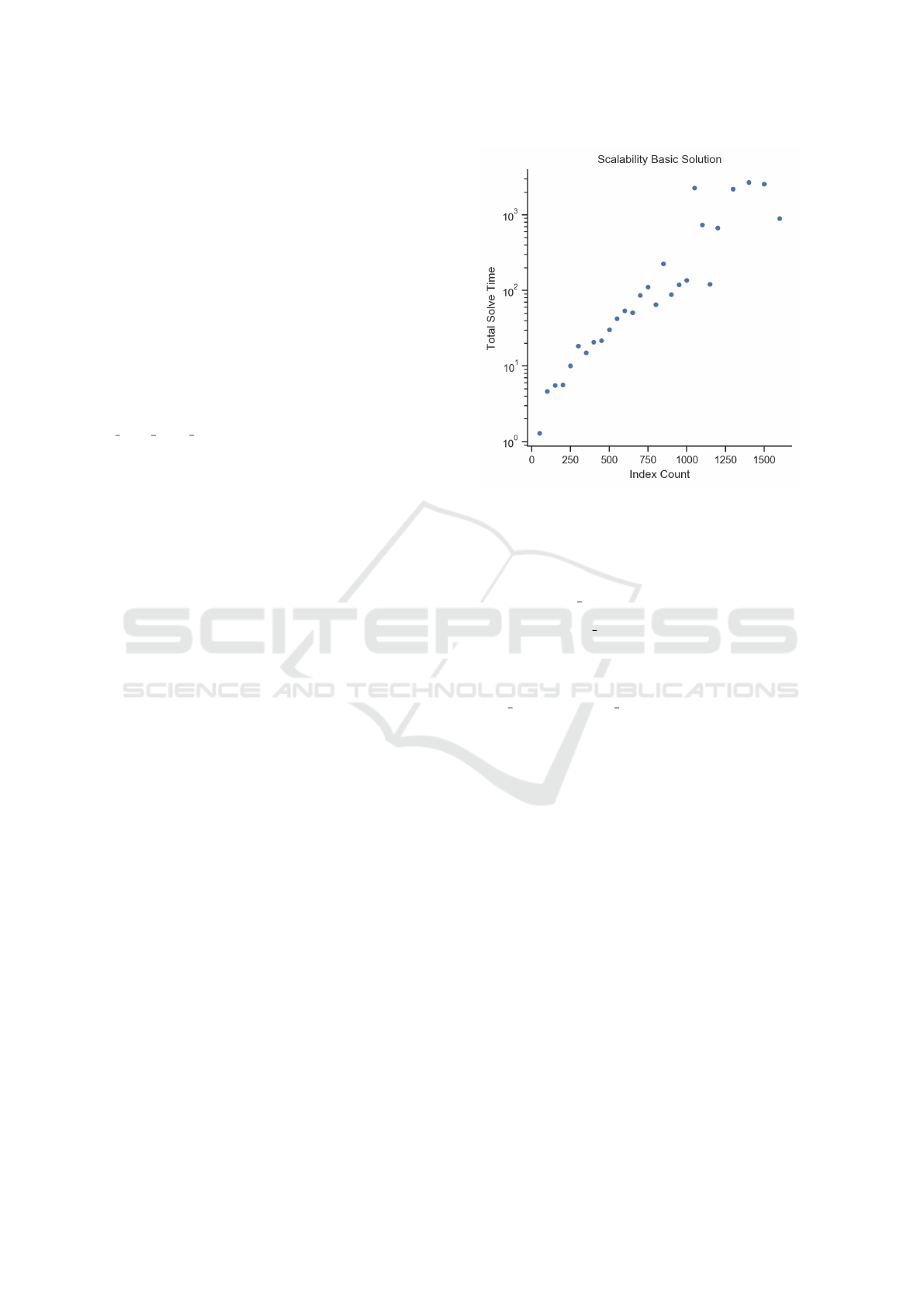
Figure 4: Execution times in seconds of the basic solution,

cf. (1) - (5), for different numbers of index candidates.

speedup s for a combination, existing of two indexes

i and j, is then calculated by the following formulas:

min speedup

i, j

= max(s

, s

) (17)

max speedup

i, j

= s

+ s

(18)

The minimum speed up and the maximum speed

up are then passed to a function that returns a uni-

formly distributed random number within the interval

[min speedup

i, j

;max speedup

i, j

], cf. (16) - (17).

Outsourcing the generation of input data into the

index-selection.data–ﬁle allows for an easy replace-

ment with actual data, e.g., benchmarking data of a

real system. However, this also enables the reader to

validate basic example cases on their own.

5.3 Basic Index Selection Solution

”The complexity of the view- and index-selection

problem is signiﬁcant and may result in high total

cost of ownership for database systems.” (Kormilitsin

et al., 2008) In this section, we evaluate our basic so-

lution, cf. Section 3.1. We show the scalability of

our implemented solution, which we later compare to

the chunking approach. We set up the memory limit

with 100 units and assume 100 queries with random

occurrences uniform between 1 and 1 000. To test the

scalability on our machine, we generate data with 50,

100, 150, ..., 1 450, 1 500 index candidates. The out-

come measurements are shown in Figure 4. The total

solve time on the y-axis is a logarithmic scale.

Figure 4 shows the growing total solve time while

the number of indexes rises. With an increasing index

ICORES 2022 - 11th International Conference on Operations Research and Enterprise Systems

count, the execution times vary more. Naturally, the

solve time depends on the speciﬁc generated data in-

put. In some cases with over 1 000 indexes, the gen-

erated input could not be solved with our setup in a

meaningful time. Note that the possible combinations

of the index selection problem grows exponentially.

In order to limit the number of index candidates, one

might only consider smaller subsets of a workload’s

queries that are responsible for the majority of the

workload costs.

5.4 Index Chunking

To tackle the exponential growing number of admis-

sible index combinations, we divide the problem into

chunks, ﬁnd the best indexes of each chunk, and then

ﬁnd the best index of the winners of all chunks, cf.

Section 3.2. Compared to the basic index selection

solution, problems with much more indexes can be

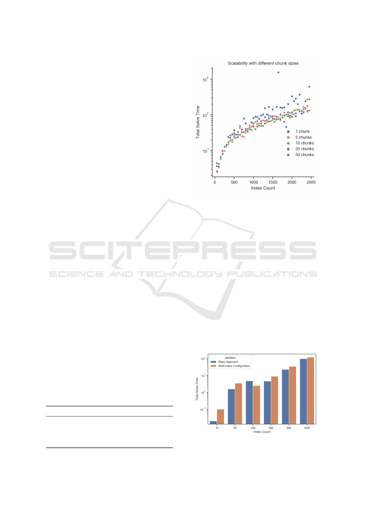
solved with chunking. Figure 5 shows the total solve

time with chunking in orange and without chunking

in blue. The other parameters were ﬁxed (see previ-

ous Section 5.3). The orange dots of the chunking

approach show a linear relationship between an in-

dex count of 500 to 2 500. In the beginning, the total

solve time of the chunking curve has a higher gradi-

ent. The overhead introduced by chunking to split the

indexes into chunks has not always a positive impact

on the total execution time of our linear program. The

chunking solution has a lower scattering than the ba-

sic solution. In each execution, some chunks could

be solved faster than the mean and some other chunks

need more time. The long and short solve times of

single chunks balance each other and chunking leads

to lower variations.

As described in Section 3.2, the heuristic chunk-

ing approach might cause the ﬁnal solution not to be

an optimal global solution of the initial problem. In

this context, Table 4 shows the total cost growth of

the found solution compared to the optimal solution.

The lower the chunk count, the higher the mean and

the maximum growth. With a lower chunk count, the

possibility that an index of the optimal solution is not

a winner of the related chunk is higher. The more

chunks, the more indexes get on to the ﬁnal round.

Table 4: Total costs growth with different numbers of

chunks compared to the optimal solution in percent (%).

# Chunks Mean growth Max growth

5 0.49 % 0.92 %

10 0.34 % 0.65 %

20 0.20 % 0.65 %

50 0.07 % 0.38 %

Figure 5: Execution times in seconds of basic solutions and

with different numbers of chunks (lower is better).

Chunking reduces the total solve time and fewer

outliers with very long execution times occur. The

degradation of the calculated solution is surprisingly

low. We observe that the total workload costs growth

is consistently lower than 1%.

5.5 Multi-index Conﬁguration

In this section, we evaluate the potential solve time

overhead, which might get introduced by the multi-

index conﬁguration extension, see Section 3.3. There-

fore, we compare the solve times of the extension with

the basic approach. For both implementations, we

tested multiple settings. The number of indexes de-

ﬁnes a setting and is one of 10, 50, 100, 200, 500, or

1 000. Independent of the setting, we assume a mem-

ory budget of 100 units and 100 queries. Figure 6

shows the solve time for both settings in comparison.

Figure 6: Execution times in seconds of the basic approach

and the multi-index conﬁguration extension in comparison.

Solver-based Approaches for Robust Multi-index Selection Problems with Stochastic Workloads and Reconﬁguration Costs

Overall, as expected, the multi-index conﬁgura-

tion extension has an execution time overhead com-

pared to the basic solution, which assigns at most only

one index to each query. However, the additional re-

quired solve time is acceptable. Further, the relative

solution time overhead decreases with an increasing

number of indexes. One explanation for this effect

could be that increasing the number of index candi-

dates also increases the number of dominated indexes

excluded by the (pre)solver.

5.6 Stochastic Workloads

In enterprise applications, we have different use cases

which produce different workloads for database sys-

tems. Each use case has different requirements. The

output of some workloads is needed within a deﬁned

time, so we could set a maximum execution time as

upper barrier for a workload. In other use cases, the

different workload costs should be robust without ma-

jor deviations. Therefore, we minimize the variance

between the costs of different workloads.

Furthermore, in other use cases, we do not need

robust workloads and the minimization of the total

costs is the best decision for database systems. In this

section, we compare different objective functions.

The next evaluated index selection problem has

I = 20 indexes, Q = 20 queries, M = 30 available

memory, and four different workloads. The W = 4

different workloads occur with different workload in-

tensities, cf. k

, see Section 3.4:

95 ×W 1 19 ×W 2 45 ×W 3 7 ×W 4 (19)

We solve this problem with the following differ-

ent optimization criteria: minimize the expected total

costs T , cf. (9), minimize the pure worst case cost L

(a −→ ∞), cf. (11), and minimize the pure variance V

(b −→ ∞), cf. (13). Note, we use these special case cri-

teria of the proposed mean-risk approaches to empha-

size their impact. For the 4th criterion, we exemplary

combine the three different criteria via the following

weighting factors, cp. (9), (11), (13):

minimize

q,i

∈{0,1}

Q×(I+1)

, L∈R

100 · T + 100 · L + 1 ·V (20)

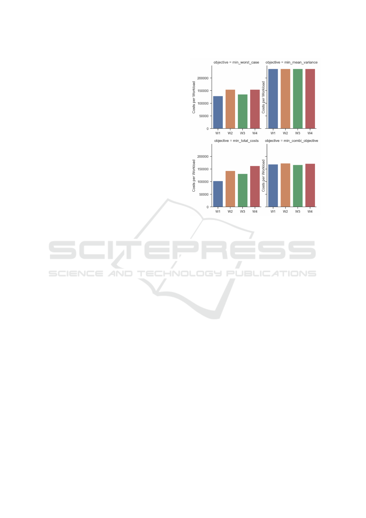
Figure 7 shows the different costs per workload

for the four objectives mentioned before. Each bar

shows the costs of one workload.

When minimizing the worst-case costs (top left

in Figure 7), the costs per workload vary between

129 017 and 154 602. When minimizing the total

costs (bottom left), the costs for each workload range

Figure 7: Workload costs with different objectives: (i) mini-

mize worst case costs L via a −→ ∞ (upper left), (ii) minimize

variance V via b −→ ∞ (upper right), (iii) minimize expected

total costs T (lower left), and (iv) the combined approach

(lower right).

from 102 907 to 162 762. The deviation between

the different workloads are higher than the workload

costs optimized with an upper barrier. The minimiza-

tion of the variance objective (top right) harmonizes

the four single workload costs. Each bar seems to

have the same height. The cost per workload is be-

tween 236 571 and 236 611. Thus, the costs for each

workload are signiﬁcantly higher than any other ap-

proach. The combination objective (bottom right)

shows a much smaller deviation than the the mini-

mization of the worst case and the total costs. With

this objective, the costs per workload are between

166 480 and 172 912.

An index selection calculated with the variance

minimization strategy leads to a fair workload cost

distribution. However, this extreme approach leads to

overall high workload costs as the mean is not part

of the objective. The problem is that workloads with

lower costs than the mean workload costs worsen

the value of the objective function. Naturally, the

quadratic objective of the BQP adds some com-

plexity. The total solve time of the pure variance

optimization was comparably large (248 s). However,

the solve time for the combined objective was only

0.78 s. Clearly, the total expected costs model and the

worst case costs model had the fastest solution times.

ICORES 2022 - 11th International Conference on Operations Research and Enterprise Systems

Table 5: Results of the four different objectives regarding

the following performance metrics: worst workload costs,

variance of the workload costs, and (expected) total costs.

Objective Worst-

case costs

Cost

variance

Total exp.

costs

worst case ∼155 k ∼8.5 G 22.4 M

variance ∼237 k 6 188 39.3 M

total exp. costs ∼163 k ∼35 G 19.5 M

combination ∼173 k ∼0.3 G 28.0 M

Table 5 shows the metrics of each optimization ap-

proach. The optimal total costs are 19 539 400. The

worst-case optimization leads to a growth of about

14.5 % compared to the total cost optimization. The

variance optimization has by far the highest total

costs, but the variance is the smallest. Compared to

the optimized variance, the worst-case optimization

has a variance that is six orders of magnitude worse,

and the total cost optimization has a variance that is

seven orders of magnitude worse. If we optimize the

worst case, we get W 4 as the worst workload with

costs of 154 602. With the total costs optimization,

the worst case is only 5 % higher. The combination

is also only 11 % higher than the minimal worst case,

but the variance approach’s worst case is 53 % higher.

The variance solution is a fair solution for all

workloads. However, for database systems, it can be

more important to execute the workloads as fast as

possible. Ultimately, it is up to the decision maker

to decide on an appropriate objective that meets the

desired outcomes.

Some workloads should be executed in a speciﬁc

time frame because a user waits on the results. In this

case, an optimization of the worst case is helpful. An-

other opportunity is to add a constraint for this single

workload to tweak the total cost optimization. How-

ever, the application needs to specify this requirement

and inform the database system in some way. If it

is not important that some workloads should be exe-

cuted within a maximum cost range, the total cost op-

timization strategy is the best one, because it reduces

the total cost of ownership of database systems.

The worst-case optimization and the total costs

optimization have similar performance indicators.

Both have their speciﬁc advantages and are good op-

timization strategies for the index selection problem.

6 FUTURE WORK

In Section 3.4, we presented alternative objectives

that minimize an upper bound to optimize the exe-

cution time of the worst workload or use the mean-

variance criterion to achieve robust execution times

with small deviations. Note that optimizing the mean-

variance criterion also penalizes execution times that

are better than the average execution time. How-

ever, short execution times are desirable from a

database perspective. Alternatively, by using mean-

semivariance criteria, one could only penalize the ex-

ecution times that are higher than the average execu-

tion time. As further risk-averse objectives also utility

functions could be used, where the associated non-

linear objectives could be resolved using piece-wise

linear approximations.

In this work, the created models were evaluated

using randomly generated synthetic data. In further

experiments, the models could also be evaluated with

data from real database scenarios to obtain more in-

formation on the quality and practical applicability of

the proposed models. For this purpose, our imple-

mentation could be executed for real database bench-

mark workloads (e.g., data of the TPC-H or TPC-DS

benchmark). A database that supports what-if opti-

mizer calls should be used to anticipate performance

improvements of the potential use of individual in-

dexes and to obtain the required model input data (i.e.,

cost values and memory consumption).

Further evaluations might further investigate the

scalability of the chunking approach as well as the

impact of (i) the assignment of similar indexes to the

same chunk and (ii) a chunk’s storage capacity, which

allows to increase or decrease the number of indexes

to be excluded, and in turn, affects both the overall so-

lution quality and the runtime. The results should al-

low to recommend storage capacities and chunk sizes

for given workloads.

Finally, our different proposed concepts and ap-

proaches should be not only compared to classical

(risk-neutral) index selection approaches (for deter-

ministic workloads) but particularly to approaches

that are also capable of addressing risk-averse objec-

tives in the presence of multiple potential future work-

loads as well as transition costs. As such evaluations

require the simulation and evaluation of more com-

plex stochastic dynamic workload realizations, we

leave such experiments to future work.

7 CONCLUSION

In this work, we considered different variants of index

selection problems and proposed solver-based solu-

tion concepts. In the basic model, we take one work-

load consisting of a set of queries and their frequen-

cies into account and decide which subset of indexes

to select under a given budget constraint.

Solver-based Approaches for Robust Multi-index Selection Problems with Stochastic Workloads and Reconﬁguration Costs

In the extended chunking approach, we divided

the overall index selection problem into multiple

smaller sub-problems, which are solved individually.

The selected indexes of these sub-problems are then

put together and the best selection among these can-

didates will be determined in a ﬁnal step. We showed

that, compared to the optimal solution of the basic

problem, this heuristic performs near-optimal and al-

lows to signiﬁcantly reduce the overall solution time.

For the multi-index conﬁguration extension, the

granularity of the possible options was changed from

the index level to the index conﬁguration level, where

each conﬁguration represents a combination of in-

dexes (e.g., a maximum of two). We showed that our

formulation is viable for standard solvers. The results

show that the execution time overhead is substantial

in small scenarios but decreases with an increasing

number of indexes.

The extension to stochastic workloads takes mul-

tiple workload scenarios into account. Such different

scenarios may be derived from historical data within

speciﬁc time spans. In this framework, different ob-

jectives were used to minimize: (1) the total workload

costs, (2) the worst-case workload costs, (3) a mean-

variance criterion, and (4) a weighted combination of

the ﬁrst three objectives. Our results show that the tar-

geted effect to avoid bad and uneven performances is

achieved.

In the fourth extension with transition costs, we

addressed the additional challenge to create and re-

move indexes in the presence of an existing conﬁgu-

ration while balancing performance and minimal re-

quired reconﬁguration costs. In our approach, we

used an extended penalty-based objective to endog-

enize creation and removal costs. We ﬁnd that in-

volving transition costs makes it possible to iden-

tify minimal-invasive reconﬁgurations of index selec-

tions, which helps to manage them over time, e.g.,

under changing workloads.

Finally, our concepts, i.e., chunking, multi-index

conﬁgurations, stochastic workloads, and transition

costs, are designed such that they can be combined.

REFERENCES

Casey, R. G. (1972). Allocation of copies of a ﬁle in an

information network. In AFIPS, pages 617–625.

Chaudhuri, S. and Narasayya, V. (2020). Anytime Algo-

rithm of Database Tuning Advisor for Microsoft SQL

Server. https://www.microsoft.com/en-us/research/

publication/anytime-algorithm-of-database-tuning-\

advisor-for-microsoft-sql-server, visited 2020-06-04.

Chaudhuri, S. and Narasayya, V. R. (1997). An efﬁcient

cost-driven index selection tool for Microsoft SQL

Server. In Proc. VLDB’97, pages 146–155.

Dash, D., Polyzotis, N., and Ailamaki, A. (2011). CoPhy:

A scalable, portable, and interactive index advisor for

large workloads. PVLDB, 4(6):362–372.

Finkelstein, S. J., Schkolnick, M., and Tiberio, P. (1988).

Physical database design for relational databases.

ACM Trans. Database Syst., 13(1):91–128.

Fourer, R., Gay, D., and Kernighan, B. (2003). AMPL: A

Modeling Language for Mathematical Programming.

Thomson/Brooks/Cole.

Kormilitsin, M., Chirkova, R., Fathi, Y., and Stallmann,

M. (2008). View and index selection for query-

performance improvement: Algorithms, heuristics

and complexity. In CIKM08: Proceedings of the 17th

ACM conference on Information and knowledge man-

agement, volume 2, pages 1329–1330.

Kossmann, J., Halfpap, S., Jankrift, M., and Schlosser, R.

(2020). Magic mirror in my hand, which is the best in

the land? An experimental evaluation of index selec-

tion algorithms. In PVLDB, volume 13, pages 2382–

2395.

Kossmann, J., Kastius, A., and Schlosser, R. (2022). Swirl:

Selection of workload-aware indexes using reinforce-

ment learning. In working paper.

Kossmann, J. and Schlosser, R. (2020). Self-driving

database systems: A conceptual approach. Distributed

and Parallel Databases, 38(4):795–817.

Papadomanolakis, S., Dash, D., and Ailamaki, A. (2007).

Efﬁcient use of the query optimizer for automated

database design. In Proc. VLDB 2007, pages 1093–

1104.

Pavlo, A. et al. (2017). Self-driving database management

systems. In CIDR 2017.

Schlosser, R. and Halfpap, S. (2020). A decomposition

approach for risk-averse index selection. In SSDBM,

pages 16:1–16:4.

Schlosser, R., Kossmann, J., and Boissier, M. (2019). Efﬁ-

cient scalable multi-attribute index selection using re-

cursive strategies. In ICDE, pages 1238–1249.

Schnaitter, K., Polyzotis, N., and Getoor, L. (2009). In-

dex interactions in physical design tuning: Modeling,

analysis, and applications. In Proc. VLDB’09, vol-

ume 2, pages 1234–1245.

Sharma, A., Schuhknecht, F. M., and Dittrich, J. (2018).

The case for automatic database administration using

deep reinforcement learning. CoRR, abs/1801.05643.

Valentin, G., Zuliani, M., Zilio, D. C., Lohman, G. M., and

Skelley, A. (2000). DB2 Advisor: An optimizer smart

enough to recommend its own indexes. In Proc. ICDE,

pages 101–110.

ICORES 2022 - 11th International Conference on Operations Research and Enterprise Systems

APPENDIX

Table 6: List of parameters and variables.

PARAMETERS

C number of index conﬁgurations

I number of indexes

M index memory budget

Q number of queries

W number of workloads

a maximum workload costs penalty factor

b variance penalty factor

c,i

binary parameter whether conﬁguration

c = 0, ..., C contains the indexes i = 1, ..., I

frequency of query q = 1, ..., Q

w,q

frequency of query q = 1, ..., Q

in workload w = 1, ..., W

intensity of workload w = 1, ..., W

memory consumption of index i = 1, ..., I

speedup of index i = 1, ..., I in contrast

to no index being used

q,i

execution time of query q = 1, ..., Q

using index i = 0, ..., I; i = 0 indicates that

no index is used

creation costs of the index i = 1, ..., I

removal costs of the index i = 1, ..., I

VARIABLES

T total expected execution time of all workloads

L maximum workload costs (worst case)

V variance of execution times

MK total creation costs

RM total removal costs

execution time of a workload w = 1, ..., W

q,c

binary variable whether conﬁguration

c = 0, ..., I is used for query q = 1, ..., Q;

c = 0 represents an empty conﬁguration

with no indexes

q,i

binary variable whether index i = 0, ..., I

is used for query q = 1, ..., Q; i = 0 indicates

that no index is used by query q

binary variable whether index i = 1, ..., I

is used for at least one query

∗

binary variable whether index i = 0, ..., I

was used previously used for at least

one query and thus is already created

Solver-based Approaches for Robust Multi-index Selection Problems with Stochastic Workloads and Reconﬁguration Costs

REFERENCES

Casey, R. G. (1972). Allocation of copies of a file in an