Spike-time Dependent Feature Clustering

Zachary S. Hutchinson

School of Computing and Information Science, University of Maine, Orono, Maine, U.S.A.

Keywords:

Dimensionality Reduction, Feature Clustering, Spiking Neural Networks, Artiﬁcial Dendrites.

Abstract:

In this paper, we present an algorithm capable of spatially encoding the relationships between elements of

a feature vector. Spike-time dependent feature clustering positions a set of points within a spherical, non-

Euclidean space using the timing of spiking neurons. The algorithm uses an Hebbian process to move feature

points. Each point is representative of an individual element of the feature vector. Relative angular distances

encode relationships within the feature vector of a particular data set. We demonstrate that trained points can

inform a feature reduction process. It is capable of clustering features whose relationships extend through time

(e.g., spike trains). In this paper, we describe the algorithm and demonstrate it on several real and artiﬁcial

data sets. This work is the ﬁrst stage of a larger effort to construct and train artiﬁcial dendritic neurons.

1 INTRODUCTION

Every data set describes a small world. The events

or objects which make up these world are typically

represented by an N-dimensional vector of features.

When N is large the shape of these worlds becomes

hard to grasp because doing so requires insight into

the N × N feature relationships which are dispersed

across all elements of the data set.

Dimensionality reduction (DR) aids in under-

standing these small worlds by reducing the number

of feature relationships. In general, DR is divided

into two areas: feature selection (FS) and feature ex-

traction (FE). FS is the process of choosing a sub-

set of the original features (Chandrashekar and Sahin,

2014). FE reduces the feature vector by casting it via

a transformation into a reduced space (Khalid et al.,

2014). The majority of DR methods rely on a mea-

surement of feature importance. This measurement

is used either in the selection process (FS) or is con-

tained within the transformation of the set of features

into a reduced space (FE).

Spike-time dependent feature clustering (SFC)

provides a new way to measure relationships between

features. SFC encodes feature relationships in the rel-

ative positions of representative points within a spher-

ical space. Hebbian learning (Hebb, 2005), driven by

individual feature values, is used to move the points

toward or away from one another. Hebbian learning is

a theory of neural plasticity which posits that changes

https://orcid.org/0000-0001-7584-0803

in the brain are in part caused by the temporal prox-

imity of two or more spikes emitted by connected

neurons. As a result, proximity within the spherical

space is the product of (dis)similarities between fea-

tures within the data set. And each feature relation-

ship dispersed throughout the data set is compressed

into a single angular distance between two points.

Once a data set is encoded, traditional clustering or

FS algorithms can be used to extract important fea-

tures. An optimal method of identifying the resulting

clusters--shape, size, or density--is beyond the scope

of this paper.

2 ALGORITHM DESCRIPTION

The clustering process uses a spiking neural network

(SNN) (Maass, 1997). A SNN consists of spiking

neurons which emit a pulse or spike when an inter-

nal value reaches a threshold. A change in input

does not immediately cause a change in neural output

but rather an output spike is a product of input over

time. Therefore, the relative timing of spikes encodes

a neuron’s recent input history. For this project, we

use the Izhikevich spiking neuron model (Izhikevich,

2007). The Izhikevich model consists an equation for

v, the membrane potential, and u, the recovery cur-

rent (Eqs. (1) and (2)). A neural spike (v ≥ v

peak

)

is modeled by a reset (v ← c, u ← u + d). The pa-

rameters used in the Izhikevich model are those given

in (Izhikevich, 2007) for a regular spiking neuron:

188

Hutchinson, Z.

Spike-time Dependent Feature Clustering.

DOI: 10.5220/0010799100003116

In Proceedings of the 14th International Conference on Agents and Artiﬁcial Intelligence (ICAART 2022) - Volume 3, pages 188-194

ISBN: 978-989-758-547-0; ISSN: 2184-433X

Figure 1: Movement across the spherical ﬁeld. Three points

(A, B, and C) correspond to three inputs. O is the ﬁeld’s

origin. A spike in A’s neuron causes A to move toward B

and C based on how recently their neurons emitted a spike.

C = 100, v

− 60, v

= −40, k = 0.7, v

peak

= 35, a =

0.03, b = −2, c = −50, d = 100.

C ˙v = k(v − v

)(v − v

) − u + I (1)

˙u = a{b(v − v

) − u} (2)

Spike-time dependent clustering utilizes a single

layer of spiking neurons. The spiking neurons trans-

form values in the examples to a time series of spikes.

Each neuron is connected to a unique point in the

spherical space. For all experiments, initial point po-

sitions are uniformly randomized over a unit shell

(identical radius). We refer to the spherical space (or

shell) occupied by the points as the ﬁeld. The dis-

tance between two points is then the angle of separa-

tion with respect to the origin (e.g., ∠AOB in Figure

1 gives the distance between A and B).

The co-activity of input neurons causes their as-

sociated points to change position. Co-activity is

deﬁned as the temporal proximity of two (or more)

spikes. Temporal proximity is a model hyperparam-

eter given by W in the equations below. In Figure

1, a spike at A causes it to move toward B and C.

The magnitude of change depends on how recently

the neurons connected to B and C have spiked. In this

example, C’s neuron has spiked more recently than

B’s. Therefore, A’s movement toward C is greater (or

∠1O2 > ∠AO1). Lastly, point 2 would give the new

location of A.

Co-activity is bounded by the learning window,

W . The learning window determines the maximum

temporal distance between two spikes that can affect

positional change. The learning window for all ex-

periments was set to 100 time steps. Furthermore,

the length of the learning window partitions measure-

ments of the ﬁeld. In other words, the learning win-

dow divides the maximum angular distance between

two points, or π, giving discrete distance markers to-

ward which points move. The goal marker of any

given instance of co-activity is the temporal distance

between two spikes. For example, if the learning win-

dow is set to 100 time steps, and one neuron routinely

spikes 50 time steps before another, the latter’s point

will move toward a location

distance away from the

former.

Point movement also depends on the sign and

strength of an error signal. For all experiments, the

error signal is within the range [−1, 1]. Negative er-

ror values cause co-activity to drive points apart (see

Equation (4)). Negative error values can be used to

separate points involved in unwanted co-activity dur-

ing a training process. Or, as they are used in several

of the following experiments, negative values can sep-

arate clusters or partition active and inactive points.

3 EXPERIMENTS

We tested the algorithm’s clustering ability on artiﬁ-

cial and real-world data sets. The goal of these exper-

iments was to discover whether point clusters formed

by the algorithm revealed underlying patterns in the

data sets. Although the types of input used across

the four experiments were different, we attempted to

make these differences invisible to the network. All

input signals were transformed into spike trains using

a Poisson process. Parameters intrinsic to the neural

and point models were identical through all experi-

ments.

Experiments 3.1 and 3.2 create patterns by using

spike trains with a similar spike rate (e.g., 100 Hz).

The spike trains themselves are randomly created by a

Poisson process. Neurons that do not belong to a pat-

tern are given a lower spike rate (e.g., 10 Hz) to sim-

ulate noise. Each input spike train is 1,000 time steps

in length. An iteration consists of one spike train

from each type of pattern and/or mask, and their order

within an iteration is random. A mask is a pattern-less

set of spike trains used in conjunction with a nega-

tive error signal to drive points away from each other.

Spikes produced by the Poisson process decayed over

time at a rate of e

−0.1t

where t is the time since the last

spike. Input spikes were scaled by a weight of 500.

3.1 Two Overlapping Patterns

For this experiment, one hundred input neurons were

divided into two overlapping patterns, A and B (see

Figure 2). Each pattern consists of ﬁfty-ﬁve 100 Hz

and forty-ﬁve 10 Hz inputs. The inputs receiving

stronger input represent the pattern and the weaker

Spike-time Dependent Feature Clustering

189

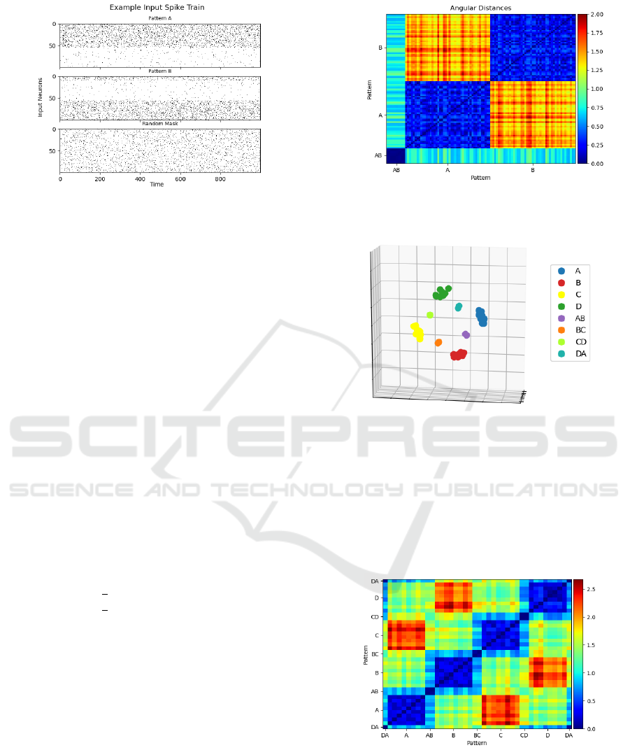
Figure 2: An example spike train for one iteration of both

patterns and the random mask. Pattern A: 100 Hz inputs

0-54, 10 Hz 55-99. Pattern B: 100 Hz inputs 0-9 and 55-99,

10 Hz 10-54. Mask: 50 Hz inputs 0-99.

inputs represent noise. Ten of the stronger 100 Hz

inputs are shared by both patterns. The network was

shown 5,000 iterations. Included in each iteration was

a random mask of identical length during which all

neurons received an input of 50 Hz.

The treatment of the mask pattern differed from

patterns A and B in that the accompanying error sig-

nal was negative (e.g., -1). For A and B, the error

value is 1. The mask was included in this (and the

following experiment) to separate clusters within the

ﬁeld.

Figure 3 shows the resulting point-by-point angu-

lar distances with points grouped by patterns along

each axis. Points unique to a pattern cluster together

(large dark blue patches). These clusters occupy dis-

joint areas of the dendritic ﬁeld (opposing warm col-

ors). The shared points form a separate cluster distinct

from the two larger clusters of unique points. The

shared cluster is approximately equidistant from the

rest of patterns A and B. Two points taken from A and

B are on average

radians from one another and the

shared points are

from the unique points. In a sim-

pliﬁed version of this experiment in which patterns A

and B are composed of disjoint sets of points, clus-

ters polarize within the ﬁeld and the distance between

points in opposing clusters is approximately π.

Shared points cause patterns to draw closer to-

gether. The greater the overlap, the closer the clus-

ters. This effect can be seen to a greater extent in the

experiment involving four overlapping patterns.

3.2 Four Overlapping Patterns

Next, we expanded the number of patterns and the

degree and complexity with which they overlapped.

Each pattern (A, B, C, and D) is comprised of twelve

neurons. Four of the twelve neurons form two pairs

Figure 3: Resulting point-point angular distances grouped

by pattern after 5,000 iterations. The overlapping points

can be seen on the bottom left.

Figure 4: Point locations after 16,000 iterations. Colors in-

dicate which pattern(s) each point belongs to.

which are shared with two other patterns (AB, BC,

CD and DA). The goal of this experiment was to in-

vestigate whether resulting clusters would themselves

cluster in such a way to resemble meta-patterns within

the input data set. All parameters were unchanged

except for the number of iterations which were in-

creased to 16,000.

Figure 5: Resulting point-point angular distances grouped

by pattern. Distance is measured in radians.

Points belonging wholly to one pattern cluster

tightly together while shared points come to rest be-

tween the clusters of their dual membership. The

meta-pattern formed by these clusters demonstrates a

kind of adjacency via shared points. Patterns which

ICAART 2022 - 14th International Conference on Agents and Artiﬁcial Intelligence

190

do not share points (i.e., A and C) oppose each other

spatially. There is a clear distinction between the av-

erage angular distance separating points of adjacent

versus non-adjacent patterns.

Several more versions of this experiment were run

which included more patterns and more complex pat-

tern overlap. Additionally, we examined whether SFC

was capable of fuzzy membership (continuous range

of rates), subpatterns (stepped rates) and additional

meta-patterns (hierarchy of rates in overlapping neu-

rons). These additional experiments reinforced the re-

sults evident in these simpler versions.

3.3 iBeacon Locations

The two previous experiments made use of artiﬁcially

generated data sets. Such sets can be large enough

to cover the relatively simple sample space of the en-

tire feature vector. To understand how well spike-time

dependent clustering works with sparse, real-world

data sets, we attempted to reproduce the placement

of iBeacons from a machine learning data set (Mo-

hammadi et al., 2017) of RSSI readings taken from

the UCI Machine Learning database (Dua and Graff,

2017).

Since SFC can train points using an unsupervised

process, we were able to use the entire data set (train-

ing and testing). We removed all entries that did not

contain two or more RSSI signals greater than the

baseline (-200). In isolation single signal entries cre-

ate no spatial association between beacons. Keeping

with the other three experiments, the order of readings

was randomized each iteration; therefore, associa-

tions between single signals could not be based on the

historical route taken through the space by the origi-

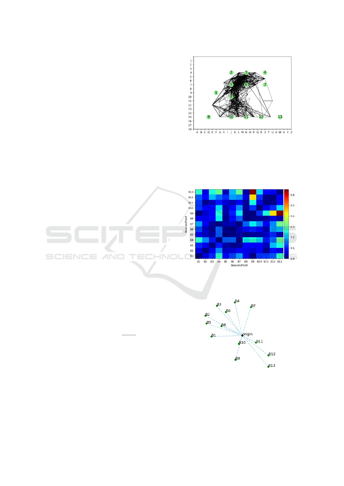
nal researcher. Figure 6 shows the grid-based place-

ment of the iBeacons from which beacon-to-beacon

distances were taken.

This modiﬁed data set was used as input to a

network with thirteen neurons (one for each bea-

con). RSSI signals were transformed into constant

rate input by the equation I

+200

200

for all b ∈

{0, 1, . . . , 12, 13} which was then used to generate an

input spike train. S

is the RSSI signal for iBeacon b

and I

is the corresponding input. An iteration con-

sisted of one full pass through the modiﬁed data set.

Between iterations entry order within the data set was

randomized.

To analyze the results we compared real-world

distances to the ﬁnal positions generated by the al-

gorithm. First, both the angular distance of points

and iBeacon Cartesian distances were normalized us-

ing min-max normalization. The absolute value of

their difference was then taken and treated as the error

Figure 6: Reproduction of the iBeacons’ physical positions

(green numbered circles) with the paths produced by en-

tries with multiple signals in both labeled and unlabeled

data sets (black lines). Indoor features of the original map

have been omitted. iBeacon positions have been adjusted

slightly to align perfectly with the nearest row and column.

Path vertices are average locations (without respect for sig-

nal strength).

Figure 7: Absolute element-wise differences of distances

between point and iBeacon positions. Point-to-point and

iBeacon-to-iBeacon distances were normalized using min-

max norm before the difference was taken.

Figure 8: Point positions within the dendritic ﬁeld result-

ing from 500 iterations. Light blue lines orient points to

the origin and give a sense of depth. Labels indicate which

iBeacon is associated with each point.

rate. Figure 7 depicts this error after 500 training iter-

ations. To establish a baseline, we generated random

Spike-time Dependent Feature Clustering

191

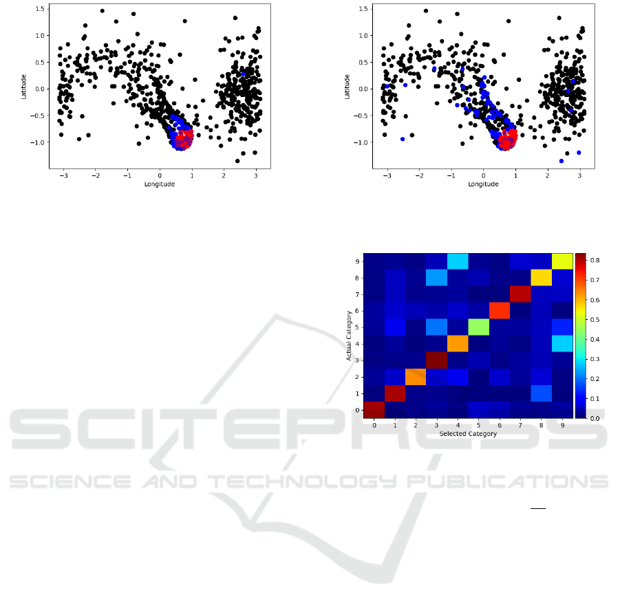
Figure 9: Digit-9 point locations. Red points indicate points

used to identify digit-9 images in the test set. Blue is the

same for digit-4. Purple are overlapping points.

point positions and compared them using the above

procedure. The error produced by random placements

(100,000 trials) had a mean of 23.7% and average me-

dian of 20.1%; whereas differences with ﬁnal point

position after 500 iterations had a mean of 10.5% and

median of 7.1%.

The relative positions of trained points roughly

correspond to actual iBeacon placement (Figure 8).

Distortions are due to examples with overlapping sig-

nals that cover either a broad (> 2 beacon signals)

or discontinuous (e.g., beacon 2 and 4 are heard but

not 3) area. The largest error between beacons 9 and

13 appears to be caused by the frequent simultane-

ous hearing of beacons 11 through 13 and the lack of

signal overlap between these and 6 and 7. The latter

is due to a lack of direct paths between 6-7 and 11-

13 owing to obstacles (see original map). The same

can be seen in the points 1 and 2 with respect to 5.

Within the indoor space, there is no direct path from

1 to 2 without passing 5; therefore, points 1, 5 and 2

form a straight line across the ﬁeld. This suggests that

the map of trained points represents obstacles as well

as iBeacon proximity and is a product of both actual

beacon location and available paths.

3.4 MNIST

How can the points of a trained ﬁeld facilitate useful

dimensionality reduction? To answer this question,

we trained ten networks on the training set of im-

ages of the MNIST handwritten image database (Le-

Cun et al., 2010) and investigated whether their points

could be used to identify the categories of testing im-

ages.

The method of training was similar to that used

to train the overlapping Poisson experiments. Image

pixel intensities were used to generate Poisson pro-

cess spike trains which were used as inputs to 784

Figure 10: Digit-9 point locations. Red dots indicate points

used to identify digit-9 images in the test set. Blue is the

same for digit-2. Purple are overlapping points.

Figure 11: Accuracy matrix showing what percent of each

image (by category) is identiﬁed as belonging to a particular

category.

neurons. Rate was determined by

255

where I

the intensity (0-255) of pixel p. Each network was

trained on the full set of testing images of a speciﬁc

category. After every ten images the networks were

shown a random mask with all inputs spiking at 50

Hz and provided an error value of -1. This caused the

inactive points to move away from clustered points.

Next we investigated whether tightly clustered

points within the trained ﬁeld could be used to rec-

ognize images from the test set. Clusters were iden-

tiﬁed by summing the angular distances of each point

to all other sibling points and selecting the N points

with the smallest summed angular distance. To ﬁnd

N, we tried several values: 20, 50, 100, 150 and 200.

N = 100 produced the best results. It is likely that

optimal results per network require a different N.

For each training image, we summed the intensi-

ties of the pixels which corresponded to the selected

points of each trained ﬁeld. The ﬁeld with the max-

imum value identiﬁed the selected category. Results

are shown in Figure 11.

The accuracy of each image category corresponds

to a degree of overlap between two sets of selected

ICAART 2022 - 14th International Conference on Agents and Artiﬁcial Intelligence

192

points. This can be seen in Figures 9 and 10. Digit-9

images were most often mistaken by this method to

be digit-4 images (27.5%) and least often to be mis-

taken as digit-2 images (0.4%). The points belong-

ing to the digit-9 and digit-4 clusters overlap signif-

icantly (Fig. 9). They share 61 points which corre-

spond to the same pixels. This stands in contrast to the

digit-9 and digit-2 clusters which share only 30 (Fig.

10). Interestingly, the non-overlapping points of digit-

9 and digit-4 clusters show a greater degree of cluster-

ing within the ﬁeld than those of digit-9 and digit-2.

The greater the overlap and lower the element-wise

inter-cluster distance the lower the accuracy due to

misidentiﬁcation.

We chose a simple cluster identiﬁcation method

(min of the sum of angular distances) for this experi-

ment to emphasize that accuracy depends on ﬁeld po-

sition and not additional cluster analysis. That said,

more complex point selection algorithms which ex-

amine the shape and size of clusters as well as degrees

of membership are likely to produce better results. As

shown in the iBeacon experiment, the shape of a clus-

ter can encode hidden information. More complex

cluster analysis is left for future work.

4 METHODS

This section gives the methods governing the move-

ment of points within the ﬁeld. The process is Heb-

bian in nature in that it is based on the relative timing

of afferent spikes.

= t

−t

(3)

in Eq. 3 gives the length of time between the

current and previous spike of neuron i. t

is the time

stamp of the current input spike received by point i.

is equivalent to the current simulation time step as

angular movement is enacted immediately. t

is the

time stamp of the previous input spike received by

point i.

+W )

−t

E (4)

Eq. 4 gives a scalar to positional change based on

the length of time between neuron i’s two most recent

spikes. W represents the effect of time. Higher val-

ues allows longer inter-spike intervals to impact point

movement. W is ﬁxed throughout the simulation at

100. Larger values slow temporal decay; smaller val-

ues increase it. t

is taken from Eq. 3. E is the cur-

rent error value which is ﬁxed at 1 (except for random

mask trials when it is set to -1). Negative values cause

co-activity to repel points.

Next, the recent activity of all sibling points is

evaluated. A copy of point i’s position,

, is orbited

toward (or away from) all sibling points to determine

the direction and magnitude of movement for point i.

For all sibling points j, where i ̸= j we calculate the

following temporal distance.

i j

= t

−t

(5)

is the time of neuron j’s most recent spike and

is the same as Eq. 3. Therefore, t

i j

measures the

interval of time between i and j’s most recent spikes.

= π

i j

(6)

represents the target angular distance between

point i and j. W is the same as given in Eq. 4. When

values of t

i j

exceed W, the point is ignored.

i j

= D

− D

(7)

i j

in Eq. 7 is the difference between the current

angular distance (D

) between points i and j and their

target angular distance (D

from Eq. 6). This and the

value of F

form the magnitude of angular change of

point i toward point j (Eq. 8).

i j

= F

i j

(8)

is then orbited across the spherical plane in the

direction of P

, the spherical position of j, by the mag-

nitude given by M

i j

Once all sibling points have been evaluated for

their effect on

, the actual position of i, P

, is

changed. P

is orbited toward

by the angular dis-

tance between them times the positional learning rate,

λ which is currently set to 0.01. This value is the re-

sult of a parameter sweep from 0.1 to 0.001.

5 DISCUSSION

Spike-time dependent clustering uses a Hebbian rule

to position points within a spherical ﬁeld. Each point

is associated with one element of a feature vector. The

relative positions of trained points encode aspects of

the set of input examples. In the iBeacon experiment,

we showed that from overlapping RSSI signals we

can reproduce the approximate layout of the beacons

themselves. And in the MNIST experiment, we can

draw out a set of representative pixels which can be

used to identify image categories.

There are a number of challenges in applying this

approach to complex data sets. First, SFC assumes

each feature has a near unique position within the

Spike-time Dependent Feature Clustering

193

overall input space. If they do not, for instance if the

centering or rotation of MNIST digits were random-

ized, SFC’s results will be much degraded. Another

process would be needed to identify bounding boxes

and rotation. Alternatively, SFC could be used to con-

struct multiple layers of ﬁelds which, similar to parts

of the visual cortex, move from simple, invariant pat-

terns (lines) into more complex ones (digits).

Another challenge is the separation of patterns or

irrelevant (or inactive) features. All experiments ex-

cept the one involving iBeacon signals used random

masks and a negative error signal to create separa-

tion. Without a separating force, inactive features

will always occupy their initial position. Clusters do

not separate on their own. Cluster orientation and

position across the spherical ﬁeld is relative. Irrele-

vant features could, by their starting position, insinu-

ate themselves into a cluster. It is our goal to ﬁnd a

method by which masks are not necessary or at least

not for this purpose. A possible solution is the in-

clusion of polarity among points. A class of negative

points would attract positive co-active points but repel

each other.

Next, the order in which points move toward other

points matters. In Figure 1, a movement ﬁrst toward

C and then B would produce a different new A. To

combat this, we randomize update order between each

iteration. The impact of update order is unknown.

However, without randomization, points have a ten-

dency to orbit the ﬁeld while maintaining relative dis-

tances.

Co-activity depends on the length of the learning

window. If it is too short, co-activity over longer inter-

vals will be missed. If the window is too long, there is

a tendency for all points to form a single cluster. The

latter also depends on the shape of the Hebbian func-

tion. One possibility is to use multiple discrete win-

dows across different networks to identify long and

short term relationships. This aspect is a challenge of

neural plasticity algorithms and credit assignment in

general.

A signiﬁcant problem in data analysis concerns

the identiﬁcation of the number of classes within a

data set. In the MNIST experiment, we presupposed

the number of classes by training ten different sets

of points and selecting one set of features from each

ﬁeld. In an unlabeled context, this is not possible.

One possibility for future research is to use SFC as a

wrapper where results from each iteration are used to

partition the data set for subsequent iterations.

In conclusion, we note that SFC is part of a larger

project to create artiﬁcial neurons with fully train-

able dendrites. Neuroscience evidence suggests that

dendritic neurons are computationally attractive (Mel,

1999). Such dendritic neurons would have expansive

dendritic trees in which synaptic (i.e., point) position,

tree shape, branch compartmentalization and synaptic

weights are all trainable parameters. Spike-time de-

pendent feature clustering describes the ﬁrst stage of

this work: synaptic position on a spherical plane. SFC

has a second part not detailed in this paper. The sec-

ond half uses co-activity of input and output neurons

to adjust the radius of a point (or synapse). In other

words, this paper describes clustering due to input-

input co-activity, while the other half describes clus-

tering due to input-output co-activity. The second half

was not included because the goal of this work was

to show that input co-activity can be used to encode

small world information in the position of synapses in

a dendritic ﬁeld.

REFERENCES

Chandrashekar, G. and Sahin, F. (2014). A survey on feature

selection methods. Computers & Electrical Engineer-

ing, 40(1):16–28.

Dua, D. and Graff, C. (2017). UCI machine learning repos-

itory.

Hebb, D. O. (2005). The organization of behavior: A neu-

ropsychological theory. Psychology Press.

Izhikevich, E. M. (2007). Dynamical systems in neuro-

science. MIT press.

Khalid, S., Khalil, T., and Nasreen, S. (2014). A survey of

feature selection and feature extraction techniques in

machine learning. In 2014 science and information

conference, pages 372–378. IEEE.

LeCun, Y., Cortes, C., and Burges, C. (2010). Mnist hand-

written digit database. ATT Labs [Online]. Available:

http://yann.lecun.com/exdb/mnist, 2.

Maass, W. (1997). Networks of spiking neurons: the third

generation of neural network models. Neural net-

works, 10(9):1659–1671.

Mel, B. W. (1999). Why have dendrites? a computational

perspective.

Mohammadi, M., Al-Fuqaha, A., Guizani, M., and Oh, J. S.

(2017). Semi-supervised Deep Reinforcement Learn-

ing in Support of IoT and Smart City Services. IEEE

Internet of Things Journal, pages 1–12.

ICAART 2022 - 14th International Conference on Agents and Artiﬁcial Intelligence

194