Towards a Better Understanding of Machine Learning based Network

Intrusion Detection Systems in Industrial Networks

Anne Borcherding

1,4 a

, Lukas Feldmann

, Markus Karch

1 b

, Ankush Meshram

2,4 c

and J

urgen Beyerer

1,2,4

Fraunhofer Institute of Optronics, System Technologies and Image Exploitation IOSB,

Fraunhofer Center for Machine Learning, Karlsruhe, Germany

Vision and Fusion Laboratory (IES), Karlsruhe Institute of Technology (KIT), Karlsruhe, Germany

Siemens AG, Germany

KASTEL Security Research Labs, Karlsruhe, Germany

Keywords:

Network Intrusion Detection, Machine Learning, Critical Infrastructure, Industrial Control Systems,

Model Inspection.

Abstract:

It is crucial in an industrial network to understand how and why a intrusion detection system detects, classiﬁes,

and reports intrusions. With the ongoing introduction of machine learning into the research area of intrusion

detection, this understanding gets even more important since the used systems often appear as a black-box

for the user and are no longer understandable in an intuitive and comprehensible way. We propose a novel

approach to understand the internal characteristics of a machine learning based network intrusion detection

system. This approach includes methods to understand which data sources the system uses, to evaluate whether

the system uses linear or non-linear classiﬁcation approaches, and to ﬁnd out which underlying machine

learning model is implemented in the system. Our evaluation on two publicly available industrial datasets

shows that the detection of the data source and the differentiation between linear and non-linear models is

possible with our approach. In addition, the identiﬁcation of the underlying machine learning model can be

accomplished with statistical signiﬁcance for non-linear models. The information made accessible by our

approach helps to develop a deeper understanding of the functioning of a network intrusion detection system,

and contributes towards developing transparent machine learning based intrusion detection approaches.

1 INTRODUCTION

Over the last decades, the realm of cybersecurity

has encountered more attacks with increasing so-

phistication than ever before. From Stuxnet to In-

dustroyer, the targets of these Advanced Persistent

Threats (APTs) vary from critical infrastructures to

industrial production systems. In order to get an

overview of cyber attacks in industrial control sys-

tems (ICS), the MITRE ATT&CK for ICS knowledge

base containing tactics, techniques, and procedures of

real threat groups can be used. To detect and address

a subset of these threats, network-based intrusion de-

tection systems (NIDSs) have become essential tools

https://orcid.org/0000-0002-8144-2382

https://orcid.org/0000-0002-5683-4499

https://orcid.org/0000-0001-6903-9446

in ICS. The objective of a NIDS is to analyze net-

work trafﬁc in order to inform the operator via alerts

and logs whenever there are indications of misuse or

abuse in the network trafﬁc. Over the last decades,

different approaches for NIDSs in industrial networks

have been proposed. One of them is the approach to

augment NIDSs with machine learning (ML) meth-

ods such as neural networks (NNs) or support vector

machines (SVMs) (Hu et al., 2018). Most of these

methods exhibit a high detection accuracy, and a low

false positive rate.

However, there are still some challenges espe-

cially with the complexity and transparency of pro-

posed ML-based NIDS since these approaches often

appear as black-box models for the user. Neverthe-

less, blue team analysts have to decide which action

to take based on the output of the NIDS. Therefore,

any credible NIDS solution must offer transparency

314

Borcherding, A., Feldmann, L., Karch, M., Meshram, A. and Beyerer, J.

Towards a Better Understanding of Machine Learning based Network Intrusion Detection Systems in Industrial Networks.

DOI: 10.5220/0010795900003120

In Proceedings of the 8th International Conference on Information Systems Security and Privacy (ICISSP 2022), pages 314-325

ISBN: 978-989-758-553-1; ISSN: 2184-4356

 2022 by SCITEPRESS – Science and Technology Publications, Lda. All r ights reserved

to the analyst in the form of visibility into the de-

tection process to understand and trust the output of

the NIDS. Transparency and reduced complexity of

the NIDS also allows the analyst to optimize deci-

sions for the judgment of the model (Sommer and

Paxson, 2010). Furthermore, governments have be-

gun to include the requirement for understanding the

reason behind the decision made by a model into leg-

islation (Amarasinghe and Manic, 2018). In order to

face these challenges and still enable the use of com-

mon ML methods such as NNs or SVMs, we propose

and evaluate a novel approach to understand the in-

ner workings of ML-based NIDS. In this context, we

assume that future vendors of commercial ML-based

NIDS solutions will not share the architecture, and

the chosen ML methods deployed. In addition, the re-

sults of this work are intended to serve as a foundation

for generating adversarial examples to enhance the ro-

bustness of NIDS solutions. We intend to bring the

attention of network-based intrusion detection system

in industrial control systems (ICS NIDSs) researchers

and vendors to the challenges encountered for trans-

parent usage of ML-based detection methods.

We suggest a model-agnostic framework to ana-

lyze ICS NIDSs in a black-box setting to improve the

understanding of the inner workings of a ML-based

NIDS. Empirically, ICS NIDSs observe the network

trafﬁc of the system under consideration over a longer

period to build their internal understanding of system

characteristics. These characteristics form the basis

for their underlying detection model. In the ﬁrst step,

we use partial dependence plots (PDPs) to determine

which data sources are used by the model under inves-

tigation. Since a NIDS can extract a variety of differ-

ent features from network traces, an analyst may ﬁrst

want to identify and understand which features have

an impact on the prediction result. In the second step,

we apply H-Statistics to determine the complexity of

the black-box NIDS. We differentiate between linear

and non-linear models providing the analyst with a

ﬁrst indicator of how complex the underlying model

is. In the last step, we use surrogate models as a

means to identify the underlying model.

We have selected the Gas Pipeline (Morris et al.,

2015) and SWaT (Mathur and Tippenhauer, 2016)

dataset fom the limited number of publicly available

ICS datasets for evaluation purposes, based on four

criteria. For each of these datasets, six different ML

models are trained. We then consider these trained

models as black-box models to evaluate our approach.

The evaluation results show that it is possible to iden-

tify the data sources, and the complexity of the model

using PDP and H-Statistics. The identiﬁcation of the

underlying model type using surrogates succeeded in

case of non-linear model types. These results are pre-

cursor to our ongoing effort of developing a frame-

work for generating adversarial examples for ICS

NIDSs to test their robustness. None of the proposed

model inspection techniques makes assumptions that

are exclusive to the domain of network intrusion de-

tection systems in industrial networks. We are con-

vinced that our approach can also be used in other

domains. To allow other researchers to reproduce our

results and to tailor the approach to their use case, we

published the source code of our implementation and

evaluation on GitHub

The rest of this paper is structured as follows. In

Section 2, we give background information on NIDS

and taxonomies for NIDS. Work related to this pa-

per is shown in Section 3. We present our approach

in Section 4 and evaluate it in Section 5. The results

of the evaluation are discussed in Section 6, and Sec-

tion 7 concludes our work.

2 REVIEW

NIST standard (Scarfone and Mell, 2007) deﬁnes

intrusion detection systems (IDSs) as software that

monitors and analyzes events occurring in a computer

system or network. For example, these events can be

log entries or ﬁle accesses, or on a network, it can be

trafﬁc patterns which are a sign of possible incidents

violating security policies or standard security prac-

tices. There are many IDS technologies differentiated

by the types of monitored events and the methodolo-

gies used to identify incidents. The most commonly

used types of IDS are NIDS and host-based intru-

sion detection systems (HIDSs). NIDSs monitor net-

work trafﬁc, and are often deployed between the con-

trol network and the corporate network in conjunction

with a ﬁrewall. In contrast to NIDSs, HIDSs mon-

itor various characteristics of the system on which

they are deployed, such as human machine inter-

face (HMI), supervisory control and data acquisition

(SCADA) servers, and engineering workstations. The

primary classes of intrusion detection methodologies

are categorized as: signature-based, compares known

threat signatures to monitored events using compari-

son operations; anomaly-based, uses statistics, expert

knowledge and ML methods to compare normal ac-

tivity against monitored events to detect signiﬁcant

deviations; and stateful protocol analysis, predeter-

mined proﬁles based on protocol standards are com-

pared against monitored events to identify deviations

from each speciﬁed protocol state activity.

https://github.com/pirofex/ml-nids-industrial-paper

Towards a Better Understanding of Machine Learning based Network Intrusion Detection Systems in Industrial Networks

315

In addition to these primary classes, different tax-

onomies for NIDS have been developed. A taxon-

omy serves the purposes of: describing a complex

observed phenomena in smaller and more manage-

able units, predicting missing entities to ﬁll up white

spots identiﬁed after classiﬁcation process and guid-

ance for explaining the observed phenomena (Axels-

son, 2000). Mitchell and Chen deﬁned ICS as a sub-

group of cyber-physical system (CPS) and introduced

a taxonomy for intrusion detection in CPS based on

two classiﬁcation dimensions: detection techniques,

what misbehavior of physical component IDS ana-

lyzes, and audit material, how IDS collects data for

analysis (Mitchell and Chen, 2014). Based on detec-

tion techniques dimension, CPS IDS are categorized

as knowledge-based, behavior-based and behavior-

speciﬁcation-based intrusion detection. Data can be

collected from CPS in two ways: host-based and

network-based auditing. Hu et al. argue that the

CPS IDS taxonomy does not take the particularity of

ICS into consideration. This particularity of ICS is

characterized by a close relationship with the physi-

cal world. They proposed a new ICS IDS taxonomy,

based on detection techniques and the characteristics

of ICS (Hu et al., 2018). The taxonomy includes

three categories: protocol analysis-based, checks vio-

lations of transmission packets in an industrial control

network against protocol speciﬁcation; trafﬁc mining-

based, analyzes nonlinear and complex relationships

between the network trafﬁc and normal/abnormal sys-

tem behaviors; and control process analysis-based,

detects semantic attacks tampering with industrial

process data or operating rules of speciﬁc control sys-

tems. Hindy et al. presented a broad taxonomy ded-

icated to the IDS design considering different char-

acteristics such as computation location, evaluation

metrics, location on the network, and detection meth-

ods (Hindy et al., 2018).

This work analyzes NIDS from a black-box point

of view, hence a novel taxonomy is developed tak-

ing the black-box perspective into account and in-

tegrating relevant characteristics drawn from estab-

lished taxonomies by Hu et al. (Hu et al., 2018) and

Hindy et al. (Hindy et al., 2018). Our proposed tax-

onomy distinguishes ICS NIDS based on three crite-

ria: detection technique, data source and model gen-

eration process. The detection technique criterion de-

scribes how a NIDS processes collected information,

and can either be signature-based or anomaly-based.

Anomaly-based detection techniques are further di-

vided into statistics-based, knowledge-based and ML-

based. ML-based techniques are further grouped

based on their model complexity as non-linear, such

as Random Forest (RF), etc., and linear, such as Lo-

gistic Regression (LR) etc.. The data source crite-

rion differentiates ICS related characteristics of data,

which has a direct impact on the features used for de-

tection, and overall monitoring range of a NIDS, into

three categories: trafﬁc mining data, includes high-

level network data like node addresses, ports, or pack-

ets sizes; protocol data, contains the protocol-speciﬁc

data which can be validated to be syntactically or se-

mantically correct; and control process data, values

of sensors and actuators in an ICS. The model gen-

eration process describes how the detection model of

NIDS reacts to changing environment in production,

either static, deployed once; or adaptive, incorporates

changes to ICS conﬁguration.

This work will focus on NIDS that are based on

ML. Hence, the corresponding subset of the taxon-

omy is shown in Figure 1. The branches and leaves

that are considered in this work are highlighted in blue

bold lines. Our approach helps to identify at which

branch and/or leaf a given black-box ML-based NIDS

is located. Identiﬁcation of linear or non-linear com-

binations of extracted features from each data source

speciﬁes the type of ICS NIDS. For example, the ICS

NIDSs specialized in control process data will uti-

lize linear/non-linear features of process data, and dif-

fer from ICS NIDSs mining network trafﬁc features.

Hence, a black-box ML-based NIDS can be catego-

rized to ICS NIDS type based on linear/non-linear us-

age of features extracted from different data sources.

3 RELATED WORK

Over the last couple of years, ML methods have

shown exceptional outcomes in a variety of ﬁelds,

such as natural language processing and computer vi-

sion. Hence, these approaches have also been widely

used in the ﬁeld of ICS NIDS. A very well-known

publicly available dataset for evaluating ML-based

ICS NIDS is the Gas Pipeline dataset (Morris et al.,

2015). Based on this dataset alone, a variety of dif-

ferent ML approaches have been compared by re-

searchers. Khan uses WEKA (Markov and Russell,

2006) to develop and deploy IDS based on Na

ıve

Bayes, PART and RF (Khan, 2019). In addition to

decision tree approaches, Sokolov et al. also con-

sidered various NN architectures, a SVM and a LR-

based classiﬁer (Sokolov et al., 2019). The algo-

rithms applied by Anton et al. are SVM, RF, k-nearest

neighbor and k-means clustering (Anton et al., 2018).

Reviewing these approaches, it can be observed that

even with the same dataset, different ML approaches

are considered and recommended.

Despite the high prediction accuracy of ML-based

ICISSP 2022 - 8th International Conference on Information Systems Security and Privacy

316

ML-based ICS NIDS

Model Type

Linear

...

Non-linear

...

Model Generation

Static

Adaptive

Data Source

Trafﬁc

Protocol

Process

Figure 1: Taxonomy for ML-based ICS NIDS from a black-box perspective. The differentiations which are part of this work

are highlighted with blue bold lines.

IDSs shown by literature, these models are more com-

plex, and the predictions of these models become

more difﬁcult to understand. In order to address these

limitations, the research ﬁeld of interpreting intrusion

detection models has transpired. Wang et al. pro-

pose an approach based on SHapley Additive exPlana-

tions (SHAP) connecting Local interpretable model-

agnostic explanations (LIME) and Shapely values to

improve the interpretation of IDS (Wang et al., 2020).

SHAP is a framework explaining the prediction of an

instance by computing the contribution of each fea-

ture. The models used to evaluate their approach were

trained on the NSL-KDD dataset (Tavallaee et al.,

2009). Marino et al. present an approach to gen-

erate explanations for incorrect classiﬁcation made

by data-driven IDS (Marino et al., 2018). The pre-

sented methodology modiﬁes a set of misclassiﬁed

samples until they are correctly classiﬁed. Amaras-

inghe and Manic suggest an approach tailored to Deep

Neural Networks (DNNs) which provides informa-

tion on the decision-making process of the DNN-IDS

for the user (Amarasinghe and Manic, 2018). The ap-

proach presented by Li et al. uses Local Explanation

Method using Nonlinear Approximation (LEMNA) to

explain the outcome of an anomaly-based IDS (Li

et al., 2019).

To the best of our knowledge, no approach focus-

ing on understanding the inner workings of ML-based

IDSs in industrial networks from a black-box perspec-

tive exists in literature. Moreover, there is only a

small amount of publications targeting the explana-

tions of the results made by ML-based NIDS in tra-

ditional IT systems (e.g. (Wang et al., 2020; Marino

et al., 2018; Amarasinghe and Manic, 2018)). Most of

these approaches make assumptions about the class of

ML models under investigation or try to describe the

inner workings using linear models. Since the com-

plexity of the models to be used in the future is not yet

apparent, we decided to use basic model inspection

techniques which have not been evaluated for ML-

based NIDS yet.

4 APPROACH

The aim of this work is to analyze ML-based NIDS,

especially with regard to their location in the taxon-

omy presented in Section 2. Similar to the taxonomy,

our approach is divided into three parts. First, we aim

to analyze the data source(s) the NIDS uses for clas-

siﬁcation. With this, we can determine which kind of

attacks are visible to the NIDS. This part of our ap-

proach is presented in Section 4.1. Second, we aim

to decide whether a given black-box NIDS is based

on a linear or non-linear model type. This informa-

tion gives insight into the complexity of the underly-

ing model type. We present this part of our approach

in Section 4.2. Third, we aim to understand which

model type is used by the NIDS in Section 4.3. This

information can build the base for further model spe-

ciﬁc investigations and analyses.

In our work, we assume that the given NIDS can

be treated as a black-box oracle. This means that there

exists no knowledge about internals of the NIDS,

especially neither the used prediction method, nor

the features which are used for the classiﬁcation are

known. Still, it is possible to send as many requests

to the models as required and access the prediction

results.

4.1 Data Source

Our main idea for the detection of the data source is

to use model inspection techniques to analyze the fea-

tures used by the NIDS. In contrast to common fea-

ture importance techniques, which try to assign a cer-

tain score to a feature, we try to detect if a feature is

recognized by a model at all. To achieve this goal,

we use PDPs (Friedman, 2000) which help to under-

stand the prediction function of a black-box model by

visualizing the dependence of a prediction result on a

set of features (Linardatos et al., 2021). To calculate

the PDP for a given feature v

, a value grid with the

observed values of the target feature is generated. For

each grid value g

i j

, one input for the NIDS is gener-

ated in which v

is set to g

i j

and all remaining features

Towards a Better Understanding of Machine Learning based Network Intrusion Detection Systems in Industrial Networks

317

−5

−2 1 2 4

0.2

0.4

0.6

0.8

Feature v

Prediction result

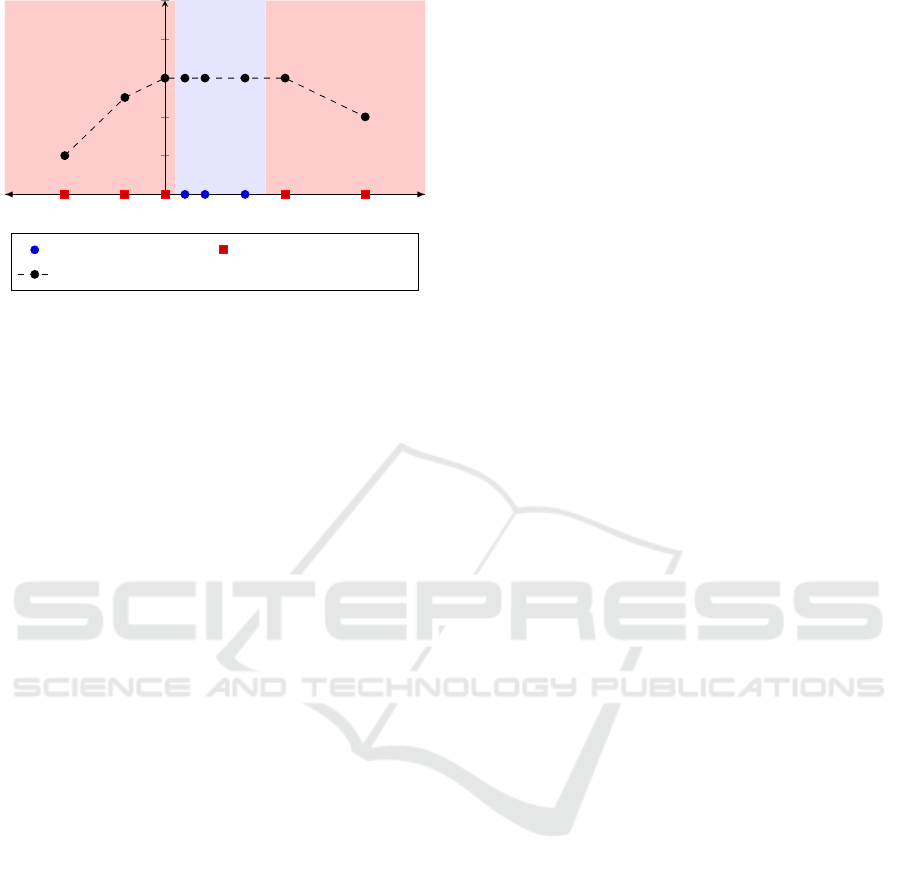
Original grid values Additional grid values

Prediction result

Figure 2: Example of a feature grid using Fibonacci sam-

pling. The feature v

has three different values from which a

Fibonacci sequence in both positive and negative directions

is sampled. With this, the impact of v

on the prediction

becomes measurable.

are set to their average. Now, the NIDS is requested

to label each of these inputs. With this, we can see

how the different values of v

inﬂuence the prediction

result. A detailed description of PDPs is given by the

original author (Friedman, 2000).

We calculate the one-way PDP for each input fea-

ture. As a result, we receive a representation of how

much the prediction result of the model changes for

different grid values of the respective feature. This is

represented as a function f , which maps a given grid

value of the feature to a prediction result of the model.

A minimal example of such a function is shown in

Figure 2. The mean absolute gradient of f shows

whether the feature has an impact on the prediction

result. If the gradient is exactly zero, we conclude

that the feature is not used by the model. If the result

is not equal to zero, the feature is deﬁnitively used by

the model. However, as it is presented in Figure 2,

with a zero gradient it is not always clear that the

feature is not recognized by the model. For exam-

ple, if the weights for a feature in a model are very

low, there might be no change in the prediction re-

sult with the values observed in the used samples. If

we would only take the observed values into account

(represented as blue circles in Figure 2), we would see

no change in the prediction result. In order to address

this issue, we propose a new method to generate the

value grid. As before, the observed values of the tar-

get features are saved in the grid (represented as blue

circles in Figure 2). In addition, the value range is ex-

tended to both sides by inserting new values that were

not present in the original data samples (represented

as red squares in Figure 2). The new values are sam-

pled using a Fibonacci sequence. With this, the re-

sulting grid contains reasonable big numbers already

after few steps. Using the additional values compen-

sates small feature weights in the model.

Finally, if the gradient of a PDP remains zero af-

ter extending the value grid, some additional veriﬁ-

cation is needed. Theoretically it might be the case

that some data points have a positive, and some have

a negative association with the prediction result, so

that they annihilate each other in a PDP. To tackle this

issue, one can use individual conditional expectation

(ICE) plots which have been presented by Goldstein

et al. (Goldstein et al., 2015). While PDPs use the av-

eraged observed changes of the prediction result, ICE

plots can be applied on each individual data point and

show how the prediction changes when the target fea-

ture changes. If the gradient of all ICE plots is zero

as well, it shows that the feature does not have any

impact on the prediction result.

4.2 Linearity

In order to make a next step towards the understand-

ing of the model type, we aim to decide whether a

given black-box NIDS is based on a linear or non-

linear model type. Intuitively, linear models are less

likely to learn dependencies between features than

non-linear models. This is why we calculate feature

interaction strengths in order to measure the degree

of non-linearity of a model. For this, H-Statistics have

been used in literature (Friedman and Popescu, 2008).

To analyze the models, we calculate H-Statistics of

all possible feature pairs in the input representation of

the models by performing the following steps for each

model M. Note that access to the original dataset is

assumed. Afterward, the resulting H-Statistics can be

compared between the different linear and non-linear

model types.

1. Sample a new dataset D of size N from the origi-

nal dataset.

2. Create a list of all two-way combinations of the

input feature representation of model M.

3. Calculate the H-Statistics for M using the samples

in D for each of these combinations.

One drawback of this approach is that the calcula-

tion of H-Statistics is computationally expensive. For

each H-Statistics computation, 2n

predictions have

to be made where n is the amount of features. De-

pending on the feature size of the dataset and the pre-

diction speed of the model type, our calculations took

a maximum of up to 16 hours, but usually less than

two hours using an Intel i7-10850H CPU with six

cores. In order to reduce the costs, it is beneﬁcial to

set the size of D as small as possible. Since marginal

distributions are estimated, there exists a certain vari-

ance. The results for the same model can differ be-

ICISSP 2022 - 8th International Conference on Information Systems Security and Privacy

318

tween two runs of creating D and calculating the H-

Statistics. To ensure that our results are not biased by

the selection of the sub-dataset, we select a sample

size at which the results are stable. For this, we eval-

uate different sample sizes and compare the standard

deviation between the different calculation rounds.

4.3 Model Type

The next step of our analysis of NIDS aims to deter-

mine the exact type of a black-box model. For this, we

train surrogate models which approximate the behav-

ior of the black-box model as proposed by Papernot

et al. (Papernot et al., 2017). Then, we use the Eu-

clidean distance of the H-Statistics as a distance met-

ric between the black-box model and the surrogates.

In detail, we calculate the Euclidean distance between

two ordered lists l and m element by element, where l

and m represent the H-Statistics of two models. This

gives us an estimation of how well the feature inter-

actions of the black-box model are approximated by

each of the surrogate models. The lower the mea-

sured distance is, the more similar the feature interac-

tion strengths are. This is why the original black-box

model is then assumed to have the same model type

as the surrogates it has the smallest distance to.

For the training of the surrogates, we propose

two different approaches. With this, we acknowledge

that there are situations where the original dataset is

known and situations in which it is not known.

Known Dataset. In our ﬁrst approach, we propose

to use the same dataset for the training of the surro-

gates that has been used for the training of the black-

box model. This assumes that the original dataset is

accessible. For practical inspection and evaluation of

NIDS this is not a huge drawback since the dataset is

known and accessible in most cases.

Unknown Dataset. In the second approach, we

propose to use the original model to create a new

dataset. This includes generating a new dataset E us-

ing general information about the input data of the

black-box model. General information can be the

type of network packets which are processed by the

model, e.g. Modbus or TCP/IP. By generating new

data packets of this type and sending them over the

network, no knowledge about the preprocessing or in-

put representation of the black-box model is needed.

Only the oracle functionality of the model is used.

Then, labels for the new dataset are created by query-

ing the original model, and the surrogates are trained

on E. For details on the packet generation for the un-

known dataset, please refer to our source code.

5 EVALUATION

In order to evaluate the three parts of our approach, we

trained different ML models on ICS network datasets

which represent different ML-based NIDS. Based on

these models, we analyze the performance of our ap-

proach. For this evaluation, we refer to the trained

NIDS as models, and the underlying ML model as

model type. To maximize the beneﬁt of the evalua-

tion, we published the source code of our evaluation.

5.1 Experimental Setup

Before we dive into the results of the evaluation, this

section clariﬁes our experimental setup. This includes

the formulation of our hypotheses, the presentation

of our strategy, and the motivation of our choice of

model types and datasets. Following this section, we

present and discuss the results of our evaluation.

5.1.1 Hypotheses

Our experiments are driven by three hypotheses

which concern the three approaches we took in order

to understand ML-based NIDS better.

H.1 The data sources a NIDS uses can be identiﬁed

using PDP and ICE plots.

H.2 H-Statistics can be used to distinguish linear

from non-linear NIDS relatively.

H.3 The model type of a NIDS can be identiﬁed

using surrogate models.

5.1.2 Strategy

To evaluate our hypotheses, we created ML models

with six model types. For each of the model types,

two models are created which are trained on one of the

two datasets respectively. These models are then used

to evaluate our approach. During our experiments,

our methods treat the models as black-box models but

are allowed to use them as oracles for an unlimited

amount of requests. That means that the models can

be asked to label a given data point for arbitrary data

points, and an arbitrary amount of times.

Similar to our hypotheses, our evaluation is di-

vided into three parts. First, we evaluate whether the

data sources used by our models can be identiﬁed us-

ing PDPs and ICE plots (Section 5.2). Second, we

evaluate the differentiation between linear and non-

linear model types (Section 5.3). Third, we evaluate

the identiﬁcation of the underlying model type (Sec-

tion 5.4)

Towards a Better Understanding of Machine Learning based Network Intrusion Detection Systems in Industrial Networks

319

5.1.3 Model Types

Based on our literature review (see Section 3), we

choose three linear and three non-linear model types

for the evaluation.

Linear models: Logistic Regression (LR),

Linear Neural Network (NN lin.), Linear Sup-

port Vector Machine (SVM lin.)

Non-linear models: Neural Network (NN),

Random Forest (RF), Support Vector Machine

(SVM).

The model type NN lin. only uses linear activation

functions in the hidden layers, and SVM lin. does not

include a kernel function. The non-linear models are

especially interesting for the differentiation of the un-

derlying model type. For each model type, one model

is trained on each of the both datasets presented in

section 5.1.4.

Note that our goal is to evaluate our proposed

techniques but not to evaluate how efﬁcient the dif-

ferent models work on the datasets. Evaluations of

the performance of different model types on ICS net-

work datasets have been conducted by different au-

thors (see Section 3). That is why we do not include

speciﬁc optimizations of the models but focus on the

evaluation of our approaches. For details on the train-

ing phase and the conﬁgurations of our models and

the surrogate models please refer to our source code.

5.1.4 Dataset

As a basis for our evaluation, we analyze different

ICS network datasets. From these datasets, we se-

lect two datasets for our evaluation. Our selection is

based on four requirements. (I) The dataset has been

evaluated in literature, and has been improved based

on these evaluations. (II) The dataset is based on a

realistic scenario in order to increase the validity of

our methods for real-world tasks. (III) A wide range

of different attacks is included in the dataset such that

models can be trained on different attack scenarios.

(IV) The dataset includes different data sources such

as trafﬁc data, protocol data, and process data such

that an evaluation regarding the identiﬁcation of data

sources used by a NIDS is feasible. The results of our

analysis of datasets based on the requirements deﬁned

above are shown in Table 1.

Based on our requirements, we choose the Gas

Pipeline dataset (Morris et al., 2015) and the SWaT

dataset (Mathur and Tippenhauer, 2016).

The Gas Pipeline dataset is based on a laboratory-

scaled gas pipeline. It consists of Modbus com-

mand/response pairs with 17 features, including traf-

ﬁc data, protocol data, and process data. Four differ-

Table 1: Evaluation of different ICS NIDS datasets regard-

ing their evaluation and enhancement by literature (Enh.),

whether they are based on a realistic scenario (Scen.), their

coverage of different attack types (Attacks), and their cov-

erage of different data sources (Data).

Dataset

Enh.

Scen.

Attacks

Data

NSL-KDD X - - -

Water Storage - X X X

SWaT X X - X

Gas Pipeline X X X X

ent attack types have been executed randomly: recon-

naissance, response injection, command injection and

denial of service. The dataset includes ﬁne-grained la-

bels for these attacks. An original version of the Gas

Pipeline dataset (Morris and Gao, 2014) has been im-

proved, and a second version of this dataset has been

published by the same authors (Morris et al., 2015)

which we use for our evaluations. In literature, both

versions of the dataset have been used for various

evaluations (eg. (Zolanvari et al., 2019; Perez et al.,

2018; Lai et al., 2019; Shirazi et al., 2016)).

The SWaT dataset is based on a scaled down ver-

sion of a real-world industrial water treatment plant

allowing data collection under two behavioral modes:

normal and attacked (Mathur and Tippenhauer, 2016).

The system consists of six stages with different fea-

tures. From the collected data, the authors created

different versions of datasets. We choose the reduced

A4&A5 dataset including three hours of SWaT under

normal operating conditions and one hour in which

six attacks were carried out. From a technical point

of view, all of these attacks are to be classiﬁed as

Man-in-the-Middle attacks, and the dataset such only

covers one attack type. In total, the dataset includes

77 features representing sensor and actuator values

from a data historian. It is important to emphasize

that NIDS solutions usually do not consider histo-

rian data as data source. Nevertheless, we decided

to select the A4&A5 SWaT dataset because we iden-

tiﬁed a high number of publications detecting anoma-

lies and cyber attacks in industrial networks based on

process data (e.g. (Inoue et al., 2017; Kravchik and

Shabtai, 2018; Lavrova et al., 2019)). The versions of

the SWaT dataset which include the original network

trace have received less attention in literature.

5.2 Data Source

In order to answer whether the used data sources can

be identiﬁed by PDP and ICE plots, we train our

models on different subsets of the datasets. For this,

we split the features of both datasets into trafﬁc data

ICISSP 2022 - 8th International Conference on Information Systems Security and Privacy

320

LR NN

NN lin.

SVM SVM lin.

function

length

crc rate

pump

1.12

0.11

2.09

9.73

0.31

4.52

1.08

0.1

1.53

8.16 · 10

−2

1.98 · 10

−3

8.24 · 10

−12

0.49

0.45

3.01 · 10

−2

8.91 · 10

−2

1.11 · 10

−16

2.27 · 10

−13

Model

Feature

Maximum absolute gradient of PDP

0.00

2.00

4.00

6.00

8.00

Gradient

Figure 3: Maximum absolute gradient of PDP for the models trained on the protocol data. The gradient has non-zero values

for used protocol data features (function, length, crc rate) and is zero for the control process feature pump not used during

training.

(high-level network features), protocol data (protocol

speciﬁc features), and process data (control process

speciﬁc features). This division is based on the prac-

tical question whether a NIDS performs deep packet

inspection and such takes process data into account.

Then, we train our models on these three subsets as

well as on the whole dataset. Afterward, we calculate

the PDP for each model as described in Section 4.1.

An extract of our results is shown in Figure 3.

The models shown on the x-axis have been trained on

the protocol data of the Gas Pipeline dataset (i.e. the

features command response, crc rate, function, and

length). For each model and each feature, we calcu-

lated the maximum gradient of the PDP. In Figure 3,

the color of each cell as well as the number displayed

in the cell corresponds to this maximum gradient. On

the y-axis three features of the protocol data as well as

an unused control process data feature (pump) is pre-

sented. It is clearly visible that the maximum gradient

helps to distinguish whether the feature has been used

by the model or not. The maximum gradient is equal

to zero for the non-used feature and is non-zero for

the used features. In the example of the ﬁgure, we can

clearly see that the models do not take the control pro-

cess data feature into account. Our experiments show

that this also holds for the other data sources (trafﬁc

and control process data). Due to space restrictions,

the ﬁgures of these experiments are not shown, but the

results can be reproduced by using the source code of

our experiments.

Our experiments support hypothesis H.1 since

they show that the gradient of the calculated plots is a

reliable indicator whether a feature has been used by

the model. From this information, it can be derived

whether the model uses trafﬁc data, protocol data, or

process data.

For our experimental setup, PDPs were sufﬁcient

NN lin.

SVM

SVM lin.

0.05

0.1

0.15

0.2

0.25

0.3

0.35

0.0373

0.2463

0.0656

0.2186

0.2485

0.0774

0.0295

0.0509

0.0373

3.2779 ·10

−3

0.058

0.0425

Model

Mean H-Statistics

Gas Pipeline SWAT

Figure 4: Mean H-Statistics of the models, grouped by

model types (incl. 95%-quantile). Linear model types

(highlighted in bold) clearly stand out relatively but not ab-

solutely.

to identify the used data source. Still, there are cases

in which an ICE plot would be needed. As discussed

in Section 4.1, if some of the data points have a pos-

itive and some have a negative association with the

prediction results, they might annihilate each other in

a PDP. In this case, an ICE plot could help to identify

the used features and such the used data source.

5.3 Linearity

After we showed how to identify the data source used

by a NIDS, we now aim to identify which underly-

ing model the NIDS uses. As a ﬁrst step, we evalu-

ate our approaches to distinguish between linear and

non-linear models. We propose to use the H-Statistics

Towards a Better Understanding of Machine Learning based Network Intrusion Detection Systems in Industrial Networks

321

to distinguish between linear and non-linear models

(see Section 4.2). In order to test the corresponding

hypothesis H.2, we conduct experiments using lin-

ear and non-linear models on both datasets (see Sec-

tion 5.1.3 for details on the models).

First, we calculate the H-Statistics for each model

and each feature pair, then use the mean of the H-

Statistics for the differentiation between linear and

non-linear model types. Figure 4 shows the calcu-

lated mean H-Statistics for all models; linear models

are printed in bold.

For the Gas Pipeline dataset, all non-linear mod-

els have relatively higher values than the linear mod-

els (see Figure 4). However, for the SWaT dataset,

this does not hold for RF. Our analysis shows that the

RF only takes few of the features into account for the

classiﬁcation. Even though it is in theory a highly

non-linear model, it behaves somewhat like a linear

model in this scenario. This is why our approach clas-

siﬁes it as a linear model, which is in fact a correct

classiﬁcation for this concrete instance of a RF.

Based on our evaluation and on our analysis of the

models, we come to the conclusion that our experi-

ments support H.2.

5.4 Surrogates

With our previous results, we are able to identify

which data source has been used, and to decide

whether a model is linear. Our next step is to identify

the underlying ML model type. For this, we are using

the approach to create surrogates and to calculate the

distance between these models using the H-Statistics

of the models presented in Section 4.3.

Known Dataset. In our ﬁrst experiment, we assume

that we do have access to the dataset that has been

used to train the original black-box model. We train

ﬁve surrogate models for each model type and cal-

culate the distances between each original model and

each surrogate model by using the H-Statistics. Each

row of Table 2 shows the mean of these distances be-

tween each model and the surrogates. The numbers

printed in bold are the minimum distance of each row,

i.e. the most likely model type for the corresponding

original model. If this minimum value lies on the di-

agonal of the matrix and such the most likely model

type is indeed the correct model type, it is highlighted

in green. If the correct identiﬁcation of the model type

was not possible, the minimum distance is highlighted

in red. Gray cells show the actual model type.

This ﬁrst analysis based on the means shows that

non-linear model types can be identiﬁed correctly.

However, the linear model types cannot be identiﬁed

based on these distances.

In addition, we perform a statistical analysis in or-

der to evaluate whether our results are signiﬁcant. For

this, we use a Mann-Whitney U Test with the alter-

native hypothesis that the distances to the surrogates

with the same model types are less than the distances

to the surrogates based on a different model type.

The resulting p-values are presented in Table 3.

It has the same structure as Table 2 but shows the

p-value for each comparison. Values that are higher

than the signiﬁcance level of 0.05 are highlighted. If

the table shows a value lower than 0.05, the model

type of the two corresponding models can be distin-

guished signiﬁcantly.

These results (presented in Table 3) show that

the model types can be distinguished from the other

model types with p-value < 0.05 for each model ex-

cept for the LR and the linear SVM. It is interest-

ing to see that the linear NN can be distinguished sig-

niﬁcantly. We perform other tests to verify this, and

the results show a statistically signiﬁcant difference in

each case.

The results in Table 2 also conﬁrm that the approx-

imation of a non-linear model is easier for non-linear

models than it is for linear models. For the non-linear

models, the distances to the non-linear surrogates are

smaller than the distances to the linear surrogates with

one exception. The approximation of the linear NN

regarding the RF is apparently better than the approx-

imation given by the NN. In addition, the linear NN

is also able to approximate LR and SVM lin. with the

lowest distance.

An additional observation is that Table 2 is not

symmetrical. This leads to the insight that the abil-

ity to approximate the model type is not symmetrical

for the linear models. For example, the distance from

a surrogate NN to the original SVMs is 3.25 whereas

the distance from a surrogate SVM to the original lin-

ear NNs is 2.92. The reason for this is the differ-

ent approximation capabilities of the different mod-

els. This difference is especially high for the linear

models which is shown by SVM lin. for example.

Our results show the SVM lin. is not suited to build

a good surrogate for the other linear models. In con-

trast, the other linear models are able to approximate

the linear SVM better. This results in the inability

to differentiate between the linear models. However,

for the non-linear models the missing symmetry is not

signiﬁcant enough to trouble the differentiation.

This experiment shows that, given the dataset, the

underlying model can be identiﬁed correctly for non-

linear model types in a statistically signiﬁcant way.

With this, it supports H.3 with the restriction to non-

linear model types.

ICISSP 2022 - 8th International Conference on Information Systems Security and Privacy

322

Table 2: Mean distance between the original models (rows) and the ﬁve trained surrogates (columns). Non-linear model types

can be identiﬁed.

LR NN NN lin. RF SVM SVM lin.

LR 0.74 3.82 0.44 2.91 3.90 3.78

NN 4.00 1.88 3.89 2.81 2.92 4.61

NN lin. 0.82 3.67 0.72 2.70 3.79 3.61

RF 2.73 2.82 2.69 0.84 2.96 3.94

SVM 4.02 3.25 4.05 3.29 2.35 4.80

SVM lin. 2.90 4.28 2.77 3.72 4.58 3.60

Table 3: Resulting p-values of a Mann-Whitney U test regarding the statistical signiﬁcance of the distance of the H-Statistics.

Non-linear model types can be distinguished signiﬁcantly (p-value < 0.05).

LR NN NN lin. RF SVM SVM lin.

LR - 0.006 0.989 0.006 0.006 0.006

NN 0.006 - 0.006 0.006 0.011 0.006

NN lin. 0.047 0.006 - 0.006 0.006 0.006

RF 0.006 0.006 0.006 - 0.006 0.006

SVM 0.006 0.006 0.006 0.006 - 0.006

SVM lin. 0.993 0.148 0.997 0.338 0.018 -

Unknown Dataset. In the second experiment, we

no longer assume access to the underlying dataset but

only the knowledge regarding the kind of data used

for the model (i.e. full network trafﬁc). With this in-

formation, we create a new labeled dataset by probing

the black-box model (see Section 4.3). Our experi-

ments show that the model type cannot be identiﬁed

in this setting. Nevertheless, this is an interesting re-

search insight.

5.5 Summary

Our experiments are driven by the three hypothe-

ses regarding the differentiation of data sources, the

differentiation between linear and non-linear models,

and the identiﬁcation of the underlying model type of

an NIDS (see Section 5.1.1). We showed with our

experiments that the data source used by our models

could be differentiated using PDPs, thus supporting

H.1. We also showed that the linearity of a model can

be assessed relatively by calculating the H-Statistics.

Thus, our experiments are supporting the hypothesis

H.2. In addition, we showed that non-linear model

types can be identiﬁed reliably using surrogates that

have been trained on the same dataset. This result

supports the hypothesis H.3 with the restriction to

non-linear model types and surrogate models trained

on the same dataset.

6 DISCUSSION AND FUTURE

WORK

Our experiments provide new insights towards a bet-

ter understanding of ML-based NIDS. The following

section discusses the results and goes into detail re-

garding possible limitations and future work.

Regarding the data source detection, our experi-

ments show that the maximum gradient of the PDP is

a good indicator to see whether a speciﬁc data source

has been used by the models. An assumption of PDPs

is that the used features are not correlated. Even

though the features of the used datasets are not com-

pletely uncorrelated (e.g. pump and pressure mea-

surement), PDPs can be used to distinguish the data

source used by the model as we compare the results

relative to each other. Nevertheless, for other datasets,

this assumption might inﬂuence the reliability of the

results.

For the differentiation between linear and non-

linear model types, we show that the differentiation

can be done relatively but not absolutely. It implies

that a decision whether a given model is linear or not

requires other known or unknown models trained on

the same, or a similar dataset. Only with those other

models, the threshold between linear and a non-linear

models can be identiﬁed.

Our experiments regarding the differentiation of

the model type show that non-linear model types can

be identiﬁed if the surrogates are trained on the same

Towards a Better Understanding of Machine Learning based Network Intrusion Detection Systems in Industrial Networks

323

dataset. For the linear model types, the differentia-

tion is not possible. In our opinion, the reason for this

lies inherently in the linearity of the models. A lin-

ear classiﬁcation might be easier to be approximated

by the other models which is why the H-Statistics are

more similar.

In addition, we showed that the differentiation

based on surrogate models trained on a re-labeled

dataset is not possible. For the practical inspection

and evaluation of NIDS this is an acceptable draw-

back since the dataset is known and accessible in most

cases since the training of the NIDS usually takes

place on-site and such the analysts have insight into

the used dataset.

During our evaluation, we identiﬁed possibilities

to extend the presented research work regarding the

coverage of the taxonomy, the performance, used

methods, and the domain. (I) Within our taxonomy

for ML-based ICS NIDS (Figure 1), the branch differ-

entiating the model generation process needs further

investigation. It would be insightful to observe how

an approach differentiates between static and adap-

tive models reliably. (II) One computationally expen-

sive part of our approach is the calculation of the H-

Statistics for all feature pair combinations. Reducing

the total amount of calculations would be a great im-

provement. This could be accomplished by weighted

feature combinations where insigniﬁcant combina-

tions are omitted. (III) As has been stated, we per-

formed no parameter tuning on the ML models we

used in our evaluation. It would be interesting to eval-

uate whether the parameter tuning and other optimiza-

tion strategies used for ICS NIDS would have an im-

pact on the results. Additionally, it would be interest-

ing to analyze which features are relevant for which

model and why. For this, our approach regarding the

data source can build a basis. (IV) In addition, instead

of H-Statistics, other methods could be used to ana-

lyze black-box models such as SHAP (Wang et al.,

2020). (V) Our approach is theoretically neither re-

stricted to NIDS nor to the domain of ICS. It would

be interesting to verify whether our approach is ap-

plicable to other domains such as HIDS, and IT net-

works. Amongst others, that could include extending

our evaluation using other datasets and model types.

7 CONCLUSIONS

We presented and evaluated approaches for a bet-

ter understanding of ML-based ICS NIDS. Our re-

sults can be set together to form a work ﬂow to an-

alyze a given black-box NIDS and test its robustness

through adversarial examples. First, one can review

the data sources used by the NIDS in order to under-

stand which kind of communication and thus which

kind of attacks are seen by the NIDS. This informa-

tion helps to understand which types of attacks are

visible to the NIDS, and which types of attacks are

not visible with no chance to be detected. Then, sur-

rogate models can be trained on the same dataset the

original model has been built on. With these surro-

gates, one can test if the black-box NIDS is a linear

or a non-linear model. This helps to understand how

complex the decision boundary of the NIDS is. With

this information, one can gain insight on how difﬁ-

cult it would be to craft adversarial examples for the

NIDS. In practice, most NIDS should use non-linear

approaches. If the black-box NIDS is indeed a non-

linear model, one can identify the model type by using

the surrogate models again. This information can then

be used to perform investigations and evaluations that

are speciﬁc for the identiﬁed model type. All those

tests and investigations lead to valuable insight into

the black-box NIDS.

We conducted our experiments in the domain of

ICS NIDS and used ICS network datasets for the eval-

uation. However, our approach is broad and funda-

mental enough to be valuable in other domains. We

want to encourage researchers in the same and in

other domains to evaluate our approach and tailor it

to their use case by using our published source code

as a basis.

ACKNOWLEDGEMENTS

This work was supported by funding from the topic

Engineering Secure Systems of the Helmholtz As-

sociation (HGF) and by KASTEL Security Research

Labs.

REFERENCES

Amarasinghe, K. and Manic, M. (2018). Improving user

trust on deep neural networks based intrusion detec-

tion systems. In IECON 2018-44th Annual Confer-

ence of the IEEE Industrial Electronics Society, pages

3262–3268. IEEE.

Anton, S. D., Kanoor, S., Fraunholz, D., and Schotten,

H. D. (2018). Evaluation of machine learning-based

anomaly detection algorithms on an industrial mod-

bus/tcp data set. In Proceedings of the 13th Interna-

tional Conference on Availability, Reliability and Se-

curity, ARES 2018, New York, NY, USA. Association

for Computing Machinery.

Axelsson, S. (2000). Intrusion detection systems: A sur-

vey and taxonomy. Technical report, Department of

ICISSP 2022 - 8th International Conference on Information Systems Security and Privacy

324

Computer Engineering, Chalmers University of Tech-

nology, G

oteborg, Sweden.

Friedman, J. (2000). Greedy function approximation: A

gradient boosting machine. The Annals of Statistics,

29.

Friedman, J. and Popescu, B. (2008). Predictive learning

via rule ensembles. The Annals of Applied Statistics,

Goldstein, A., Kapelner, A., Bleich, J., and Pitkin, E.

(2015). Peeking inside the black box: Visualizing

statistical learning with plots of individual conditional

expectation. journal of Computational and Graphical

Statistics, 24(1):44–65.

Hindy, H., Brosset, D., Bayne, E., Seeam, A., Tachtatzis,

C., Atkinson, R., and Bellekens, X. (2018). A taxon-

omy and survey of intrusion detection system design

techniques, network threats and datasets. Technical

report, University of Strathclyde, Glasgow.

Hu, Y., Yang, A., Li, H., Sun, Y., and Sun, L. (2018). A

survey of intrusion detection on industrial control sys-

tems. International Journal of Distributed Sensor Net-

works, 14(8):1550147718794615.

Inoue, J., Yamagata, Y., Chen, Y., Poskitt, C. M., and Sun,

J. (2017). Anomaly detection for a water treatment

system using unsupervised machine learning. In 2017

IEEE international conference on data mining work-

shops (ICDMW), pages 1058–1065. IEEE.

Khan, A. A. Z. (2019). Misuse intrusion detection using

machine learning for gas pipeline scada networks. In

Proceedings of the International Conference on Secu-

rity and Management (SAM), pages 84–90.

Kravchik, M. and Shabtai, A. (2018). Detecting cyber at-

tacks in industrial control systems using convolutional

neural networks. In Proceedings of the 2018 Work-

shop on Cyber-Physical Systems Security and Pri-

vaCy, pages 72–83.

Lai, Y., Zhang, J., and Liu, Z. (2019). Industrial anomaly

detection and attack classiﬁcation method based on

convolutional neural network. Security and Commu-

nication Networks, 2019.

Lavrova, D., Zegzhda, D., and Yarmak, A. (2019). Using

gru neural network for cyber-attack detection in auto-

mated process control systems. In 2019 IEEE Interna-

tional Black Sea Conference on Communications and

Networking (BlackSeaCom), pages 1–3. IEEE.

Li, H., Wei, F., and Hu, H. (2019). Enabling dynamic net-

work access control with anomaly-based ids and sdn.

In Proceedings of the ACM International Workshop

on Security in Software Deﬁned Networks & Network

Function Virtualization, pages 13–16.

Linardatos, P., Papastefanopoulos, V., and Kotsiantis, S.

(2021). Explainable ai: A review of machine learn-

ing interpretability methods. Entropy, 23(1):18.

Marino, D. L., Wickramasinghe, C. S., and Manic, M.

(2018). An adversarial approach for explainable ai in

intrusion detection systems. In 44th Annual Confer-

ence of the IEEE Industrial Electronics Society, pages

3237–3243. IEEE.

Markov, Z. and Russell, I. (2006). An introduction to the

weka data mining system. ACM SIGCSE Bulletin,

38(3):367–368.

Mathur, A. P. and Tippenhauer, N. O. (2016). Swat: a wa-

ter treatment testbed for research and training on ics

security. In 2016 International Workshop on Cyber-

physical Systems for Smart Water Networks, pages

31–36. IEEE.

Mitchell, R. and Chen, I.-R. (2014). A survey of intrusion

detection techniques for cyber-physical systems. ACM

Computing Surveys (CSUR), 46(4):1–29.

Morris, T. and Gao, W. (2014). Industrial control system

trafﬁc data sets for intrusion detection research. In In-

ternational Conference on Critical Infrastructure Pro-

tection, pages 65–78. Springer.

Morris, T. H., Thornton, Z., and Turnipseed, I. (2015). In-

dustrial control system simulation and data logging

for intrusion detection system research. 7th annual

southeastern cyber security summit, pages 3–4.

Papernot, N., McDaniel, P., Goodfellow, I., Jha, S., Celik,

Z. B., and Swami, A. (2017). Practical black-box at-

tacks against machine learning.

Perez, R. L., Adamsky, F., Soua, R., and Engel, T. (2018).

Machine learning for reliable network attack detection

in scada systems. In 2018 17th IEEE International

Conference On Trust, Security And Privacy In Com-

puting And Communications/12th IEEE International

Conference On Big Data Science And Engineering

(TrustCom/BigDataSE), pages 633–638. IEEE.

Scarfone, K. and Mell, P. (2007). Guide to intrusion de-

tection and prevention systems (idps). NIST special

publication, 800(2007):94.

Shirazi, S. N., Gouglidis, A., Syeda, K. N., Simpson, S.,

Mauthe, A., Stephanakis, I. M., and Hutchison, D.

(2016). Evaluation of anomaly detection techniques

for scada communication resilience. In 2016 Re-

silience Week (RWS), pages 140–145. IEEE.

Sokolov, A. N., Pyatnitsky, I. A., and Alabugin, S. K.

(2019). Applying methods of machine learning in the

task of intrusion detection based on the analysis of in-

dustrial process state and ics networking. FME Trans-

actions, 47(4):782–789.

Sommer, R. and Paxson, V. (2010). Outside the closed

world: On using machine learning for network intru-

sion detection. In 2010 IEEE Symposium on Security

and Privacy, pages 305–316.

Tavallaee, M., Bagheri, E., Lu, W., and Ghorbani, A. A.

(2009). A detailed analysis of the kdd cup 99 data

set. In 2009 IEEE symposium on computational intel-

ligence for security and defense applications, pages

1–6. IEEE.

Wang, M., Zheng, K., Yang, Y., and Wang, X. (2020). An

explainable machine learning framework for intrusion

detection systems. IEEE Access, 8:73127–73141.

Zolanvari, M., Teixeira, M. A., Gupta, L., Khan, K. M.,

and Jain, R. (2019). Machine learning-based network

vulnerability analysis of industrial internet of things.

IEEE Internet of Things Journal, 6(4):6822–6834.

Towards a Better Understanding of Machine Learning based Network Intrusion Detection Systems in Industrial Networks

325