Automated Information Leakage Detection: A New Method Combining

Machine Learning and Hypothesis Testing with an Application to

Side-channel Detection in Cryptographic Protocols

Pritha Gupta

1 a

, Arunselvan Ramaswamy

1 b

, Jan Peter Drees

2 c

, Eyke H

ullermeier

3 d

Claudia Priesterjahn

4 e

and Tibor Jager

2 f

Department of Computer Science, Paderborn University, Warburger Str. 100, 33098 Paderborn, Germany

Department of Computing, University of Wuppertal, Gaußstraße 20, 42119 Wuppertal, Germany

Institute of Informatics, University of Munich (LMU), Akademiestr. 7, 80538 Munich, Germany

achelos GmbH, Vattmannstraße 1, 33100 Paderborn, Germany

Keywords:

Information Leakage, Side-channel Attacks, Statistical Tests, Supervised Learning.

Abstract:

Due to the proliferation of a large amount of publicly available data, information leakage (IL) has become a

major problem. IL occurs when secret (sensitive) information of a system is inadvertently disclosed to unau-

thorized parties through externally observable information. Standard statistical approaches estimate the mutual

information between observable (input) and secret information (output), which tends to be a difﬁcult problem

for high-dimensional input. Current approaches based on (supervised) machine learning using the accuracy

of predictive models on extracted system input and output have proven to be more effective in detecting these

leakages. However, these approaches are domain-speciﬁc and fail to account for imbalance in the dataset.

In this paper, we present a robust autonomous approach to detecting IL, which blends machine learning and

statistical techniques, to overcome these shortcomings. We propose to use Fisher’s Exact Test (FET) on the

evaluated confusion matrix, which inherently takes the imbalances in the dataset into account. As a use case,

we consider the problem of detecting padding side-channels or ILs in systems implementing cryptographic

protocols. In an extensive experimental study on detecting ILs in synthetic and real-world scenarios, our ap-

proach outperforms the state of the art.

1 INTRODUCTION

Information leakage (IL) is termed as the unintended

disclosure of the sensitive information to an unautho-

rized person or an eavesdropper via observable sys-

tem information (Hettwer et al., 2020). Detecting

these ILs is crucial since they can cause electrical

blackouts, theft of valuable and sensitive data like

medical records and national security secrets (Het-

twer et al., 2020). The task of detecting IL in a given

system is called information leakage detection (ILD).

A system, intentionally or inadvertently, releases

https://orcid.org/0000-0002-7277-4633

https://orcid.org/0000-0001-7547-8111

https://orcid.org/0000-0002-7982-9908

https://orcid.org/0000-0002-9944-4108

https://orcid.org/0000-0001-7236-9411

https://orcid.org/0000-0002-3205-7699

huge amounts of information publicly, which can

be recorded by any outside observer called the ob-

servable information (data). Precisely, IL occurs in

this system if the observable information is directly

or indirectly correlated to secret information (secret

keys, plaintexts) of the system, which may result in

compromising the security. Most current approaches

based on statistics estimate the mutual information

between observable and secret information to quan-

tify IL. However, these estimates suffer from the

problem of the curse of dimensionality of inputs (ob-

servable information) and in addition, strongly rely

upon time-consuming manual analysis by domain ex-

perts (Chatzikokolakis et al., 2010). Current state-of-

the-art research focuses on the development and ap-

plication of machine learning for ILD since they have

been proven to be more effective (Moos et al., 2021;

Mushtaq et al., 2018). These approaches analyze the

152

Gupta, P., Ramaswamy, A., Drees, J., Hüllermeier, E., Priesterjahn, C. and Jager, T.

Automated Information Leakage Detection: A New Method Combining Machine Learning and Hypothesis Testing with an Application to Side-channel Detection in Cryptographic Protocols.

DOI: 10.5220/0010793000003116

In Proceedings of the 14th International Conference on Agents and Artiﬁcial Intelligence (ICAART 2022) - Volume 2, pages 152-163

ISBN: 978-989-758-547-0; ISSN: 2184-433X

accuracy of the supervised learning model on the data

extracted from the given system, by using the observ-

able information as input and the secret information

as the output (Moos et al., 2021). However, these

approaches are domain-speciﬁc and not equipped to

handle the imbalanced datasets, making them possi-

bly miss novel ILs (false negatives) or detect non-

existent leakage in the system (false positives) (Picek

et al., 2018). Our approach tackles this problem by

using the weighted version of supervised learning al-

gorithms and the evaluated confusion matrix to de-

tect the IL which inherently takes the imbalance in

the dataset into account (Hashemi and Karimi, 2018).

As a use-case, we consider the problem of side-

channel detection in cryptographic systems, which

is an application of ILD. A cryptographic system

unintentionally releases the observable information

via many modes, such as network messages, CPU

caches, power consumption, or electromagnetic radi-

ation. These modes are exploited by the side-channel

attacks (SCAs) to reveal the secret inputs (informa-

tion) to an adversary, potentially rendering all im-

plemented cryptographic protections irrelevant (Moos

et al., 2021; Mushtaq et al., 2018). A system is

said to contain a side-channel, if there exists a SCA

which can reveal secret keys (or plain-texts), mak-

ing it vulnerable. The existence of a side-channel

in a cybersecurity system is equivalent to the occur-

rence of IL. In this ﬁeld, the most relevant literature

uses machine learning to perform SCAs, not prevent-

ing side-channels through early detection of ILs (Het-

twer et al., 2020). Current machine learning-based

approaches are able to detect side-channels, thus pre-

venting SCA on the algorithmic and hardware levels

and this has been presented by Zhang et al. (2020);

Perianin et al. (2021); Mushtaq et al. (2018). These

approaches apply the supervised-learning techniques

using the observable system information as input to

classify a system as vulnerable (with IL) or non-

vulnerable (without IL). For generating the binary

classiﬁcation datasets, they extracted observable in-

formation from the secured systems as input, label

them as 0 (non-vulnerable) and then introduce known

ILs in these systems and label them 1 (vulnerable).

This process makes these approaches domain-speciﬁc

and misses novel side-channels (Perianin et al., 2021).

Current state-of-the-art automated learning-based

approaches improve this by analyzing the accuracy of

supervised-learning models on the binary classiﬁca-

tion data extracted from the given system, such that

observable information is used as input and partial

(sensitive) information is used as output (Moos et al.,

2021; Drees et al., 2021). These approaches are re-

stricted to detecting side-channels accurately, only if

the extracted data is balanced, not noisy, and also pro-

duces a large number of false positives. The problem

of imbalanced, noisy system datasets is very common

in real-life scenarios (Zhang et al., 2020).

Our Contributions. We propose a novel approach

that provides a general solution for detecting IL by

testing the learnability of the binary classiﬁers on

the extracted binary classiﬁcation data from the sys-

tem. To account for imbalance in the dataset we use

weighted versions of the binary classiﬁers and test

the evaluated confusion matrices using Fisher’s Ex-

act Test (FET) (Hashemi and Karimi, 2018). The

FET inherently takes the imbalance into account by

indirectly using the Mathews Correlation Coefﬁcient

evaluation measure, which is zero if the predictions

are obtained by guessing the label (random guessing)

or predicting the majority label (majority voting clas-

siﬁer) (Chicco et al., 2021). To account for the noise,

we deﬁne an ensemble of binary classiﬁers which in-

cludes a Deep multi-layer perceptron and aggregate

their FET results (p-values) to get the ﬁnal verdict on

the IL in a system. We show that our approach is more

efﬁcient (detection time) and accurate in detecting

side-channels in real-world cryptographic OpenSSL

TLS protocol implementations and ILs in synthetic

scenarios as compared to the current state-of-the-art.

2 INFORMATION LEAKAGE:

PROBLEM FORMULATION

In this section, we formalize the condition for occur-

rence information leakage (IL) in a given system us-

ing the binary classiﬁcation problem described in the

Appendix. We also deﬁne the information leakage de-

tection (ILD) task using a mapping, which classiﬁes

the given system as vulnerable and non-vulnerable.

2.1 Information Leakage

IL occurs in a system (extracted data D) when ob-

servable information (data) X is directly or indirectly

correlated to secret information (secret keys, plain-

texts) Y of the system, i.e., there is some informa-

tion present in the X that can be used to derive the

label y. The observable data is used as input (X ) and

the secret information as the output (Y ) for the binary

classiﬁcation algorithms, which produces a mapping

ˆg between them, produced by Equation (5) deﬁned in

the Appendix.

In the following, we suggest using the Bayes pre-

dictor g

, to check for dependencies (correlation) be-

tween X and Y , thus for IL in a system. The (point-

Automated Information Leakage Detection: A New Method Combining Machine Learning and Hypothesis Testing with an Application to

Side-channel Detection in Cryptographic Protocols

153

wise) Bayes predictor g

minimizes the expected 0-1

loss (L

) of the prediction ˆy for given input x:

(x) = arg min

ˆy∈Y

∑

y∈Y

( ˆy,y) p(y|x)

= arg min

ˆy∈Y

( ˆy,y)|x], (1)

where E

] is the expected 0-1 loss with respect to

y ∈Y and p(y|x) is the conditional probability of the

class y given an instance x. If X and Y are indepen-

dent of each other then, p(y|x) = p(y), such that p(y)

corresponds to the prior distribution of y, then g

deﬁned as:

(x) = arg max

y∈Y

p(y) (2)

For every point x ∈ X , g

predicts label 0 if p(1) <

p(0) and label 1 if p(1) > p(0), which implies the

Bayes predictor is a majority voting classiﬁer, when

p(y|x) = p(y). Hence, if g

produces an 0-1 loss less

than the 0-1 loss of majority voting classiﬁer, then

there exists a dependency between X and Y . For a

known distribution p(y|x), if g

produces a loss (sig-

niﬁcantly) lower than that of a majority voting classi-

ﬁer, we imply that IL occurs in the system, else not.

In reality, only D is available, so in place of Bayes

Predictor, we use the empirical risk minimizer ˆg pro-

duced by minimizing Equation (5). Using this, we

quantify the IL in a system as the difference between

average 0-1 loss (1−m

ACC

) for ˆg and majority voting

classiﬁer. If this difference is signiﬁcant enough, then

we conclude that IL occurs in the given system (that

generates D). This condition is the basis for our ILD

approaches proposed in Section 3.

2.2 Information Leakage Function

The problem of ILD is reduced to analyzing the learn-

ability of these binary classiﬁers on the given dataset.

In a nutshell, we test this by hypothesizing that if the

mapping produced by the supervised learning algo-

rithm, accurately predicts the outputs using the inputs,

then the correlation between the input and output is

high, which implies the existence of IL in the system.

The task of an ILD approach is to assign a label

to the extracted dataset D from a system, such that

0 indicates occurrence and 1 indicates the absence of

IL in the system. Let D be the binary classiﬁcation

data extracted from the system, such that the observ-

able information is represented by inputs X ⊂ R

and

secret-information by outputs Y = {0,1}. Given a

dataset D of size N, the task of detecting IL boils

down to associating D with a label in {0, 1}, where

0 suggests “no information leakage” and 1 suggests

“information leakage”. Thus, we are interested in the

function I deﬁned as:

I :

[

N∈N

(X ×Y )

→ {0,1}, (3)

which takes a dataset D (extracted from the system)

of any size as input and returns an assessment of the

possible existence of IL in the given system as an out-

put. We denote the mapping

I as the predicted IL

function produced by an ILD approach.

IL-Dataset. Let L = {(D

)}

i=1

be the IL-

Dataset, such that N

∈ N,z

∈ {0,1}, ∀i ∈ [N

] Let

z = (z

,... , z

) be the ground-truth vector, gener-

ated by the I, such that z

= I(D

),∀i ∈ [N

]. Let

ˆz = (ˆz

,... , ˆz

) be the corresponding prediction vec-

tor, such that ˆz

I(D

),∀i ∈[N

]. Since the ILD task

produces binary decisions, their accuracy is measured

using the binary classiﬁcation evaluation metrics, e.g.

accuracy for the ground-truth z and predictions ˆz is

calculated using m

ACC

(z, ˆz) as described in the Ap-

pendix. To avoid confusion, we will refer to L as IL-

Dataset and each D as the dataset.

3 INFORMATION LEAKAGE

DETECTION: OUR

APPROACHES

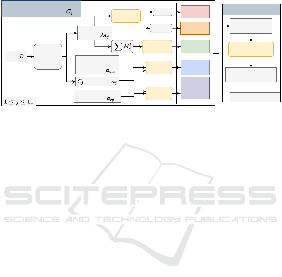
In this section, we describe our proposed information

leakage detection (ILD) approaches using binary clas-

siﬁcation and statistical tests as shown in Figure 1. In

addition, we describe an aggregation method based on

using a set of binary classiﬁers and Holm-Bonferroni

Correction to make our approaches more robust.

3.1 Paired T-Test based Approach

From the machine learning perspective, information

leakage (IL) occurs in a system, if a binary classiﬁ-

cation algorithm trained on the dataset extracted from

the system produces an accurate mapping between in-

put (observable information) and output (secret infor-

mation). This accuracy should be signiﬁcantly bet-

ter than that of the Bayes predictor evaluated on the

dataset extracted from a secure system. For such sys-

tems, the inputs and outputs are independent of each

other and Bayes predictor becomes majority voting

classiﬁer as per Equation (2) deﬁned in the Appendix.

This provides us motivation to use paired statis-

tical tests between the performance estimates, i.e.,

K accuracies obtained from K-Fold cross-validation

(KFCV) of the binary classiﬁer and majority voting

classiﬁer. These tests examine the probability (p-

value) of observing the statistically signiﬁcant differ-

ence between the paired samples (accuracies of ma-

jority voting classiﬁer and binary classiﬁer) (Dem

sar,

2006). The p-value is the probability of obtaining

ICAART 2022 - 14th International Conference on Agents and Artiﬁcial Intelligence

154

Aggregation

Decision on

Information Leakage

P-values

of 11 Classifiers

Holm-Bonferroni

Correction

Confusion

Matrices

Fisher's

Exact-Test

FET-SUM

FET-MEAN

FET-

MEDIAN

Derivation of p-value from each

approach for Classifier

Accuracies

Majority Voting

Classifier

Accuracies

K-Fold

Nested

Cross-

Validation

Data

Paired

T-Test

Fisher's

Exact-Test

Mean

Median

Random Guessing

Accuracies

PTT-

MAJORITY

PTT-

RANDOM

(Baseline)

Paired

T-Test

For Each Approach

Figure 1: Approaches for Information Leakage Detection.

test results (mean of the difference between the ac-

curacies) at least as extreme as the observation, as-

suming that the null hypothesis (H

) is true (Dem

sar,

2006). The null hypothesis H

states that the accu-

racies are drawn from the same distribution (no dif-

ference in performance) or the average difference be-

tween the paired samples drawn from the two popula-

tions is zero(∼ 0) (Dem

sar, 2006).

Out of many paired statistical tests, the most com-

monly used paired tests are the Paired T-Test (PTT)

and the Wilcoxon-Signed Rank test (Dem

sar, 2006).

These tests assume that each accuracy estimate is

independent of each other and using KFCV vio-

lates the assumption of independence (the training

data across each fold overlaps). Nadeau and Bengio

(2003) showed that the violation of independence in

the paired tests leads to overestimating the t statis-

tic, resulting in tests being optimistically biased. We

consequently choose to use their corrected version of

the PTT, because it accounts for the dependency in

KFCV, as explained in the Appendix.

The shortcoming of PTT is their asymptotic na-

ture and the assumption that the samples (difference

between the accuracies) are normally distributed,

which results in optimistically biased p-values. This

approach is based on accuracy, which is an ex-

tremely misleading metric for imbalanced classiﬁca-

tion datasets (Powers, 2011; Picek et al., 2018).

3.2 Fisher’s Exact Test based Approach

To address the problem of class-imbalance and incor-

rect p-value estimation, we propose to use Fisher’s

Exact Test (FET) on the evaluated K confusion ma-

trices (using KFCV) to detect IL.

IL is likely to occur if there exists a (sufﬁciently

strong) correlation between the inputs x and the out-

puts y in the given data D. The predictions produced

by the classiﬁer C

is deﬁned as ˆg(x) = ˆy, where ˆg is

the predicted function as per Equation (5) deﬁned in

the Appendix. So, ˆy is seen as single point encapsu-

lating the complete information contained in the input

x. If there exists a correlation, then ˆy will contain in-

put information that is relevant/used for predicting the

correct outputs (TP,TN). We can therefore determine

the existence of IL by examining the dependency be-

tween predictions ˆy

of C

and the ground-truths y.

We proposed to apply FET on the confusion ma-

trix for calculating the probability of independence

between the model predictions ˆy and the actual labels

y (Fisher, 1922). FET is a non-parametric test that

is used to calculate the probability of independence

(non-dependence) between two classiﬁcation meth-

ods, in this case, classiﬁcation of instances according

to ground-truth y and the binary classiﬁer predictions

ˆy (Fisher, 1922). The null hypothesis H

states that

the model predictions ˆy and ground-truth labels y are

independent, implying absence of IL. While the alter-

nate hypothesis H

states that the model predictions

ˆy are (signiﬁcantly) dependent on the ground-truth la-

bels y, implying occurrence of IL.

The advantage of using FET is that the p-value

is calculated using Hypergeometric distribution ex-

actly, rather than relying on an approximation that be-

comes exact in the limit with sample size approach-

ing inﬁnity, as is the case for many other statistical

tests. In addition to that, this approach directly tests

the learnability of a binary classiﬁer (without con-

sidering majority voting classiﬁer) and is indirectly

proportional to the Mathews Correlation Coefﬁcient

performance measure, which takes class-imbalance in

the dataset into account (Camilli, 1995; Chicco et al.,

2021). Please refer to the Appendix for details.

Automated Information Leakage Detection: A New Method Combining Machine Learning and Hypothesis Testing with an Application to

Side-channel Detection in Cryptographic Protocols

155

3.3 On Robustness

For making our ILD approaches more robust, we de-

ﬁne a set of 11 binary classiﬁers C that are evaluated

on the extracted dataset D of the given system.

The motivation of using an ensemble of binary

classiﬁers, rather than just one binary classiﬁer is that

each binary classiﬁer restricts their hypothesis space

H , based on the assumptions imposed on h. In addi-

tion, the statistical tests are asymmetric in nature, i.e.

they can only be used to reject H

which implies that

we can prove the existence of IL but not its absence.

To work around both restrictions, we use a set of mul-

tiple binary classiﬁers (C ,|C |= 11) to detect IL more

reliably inculcating greater trust in the absence of IL,

if all classiﬁers fail to ﬁnd an accurate matching.

The set of binary classiﬁers C (|C | = 11), in-

cludes simple and commonly used linear classiﬁers,

which assume linear dependencies between the input

and output, such as Perceptron, Logistic Regression,

and Ridge Classiﬁer. C also includes Support Vector

Machine, which classiﬁes the non-linearly separable

data using a kernel trick, i.e. its hypothesis space also

contains non-linear functions. C also includes Deci-

sion Tree and Extra Tree, which learn a set of rules

using a tree for classiﬁcation (Geurts et al., 2006). To

learn more complex dependencies with very high ac-

curacy, we also include ensemble based binary classi-

ﬁers in C . The ensemble based approaches train mul-

tiple binary classiﬁers (base learners) on the given

dataset and the ﬁnal prediction is obtained by aggre-

gating the predictions of each base learner. The two

most popular approaches proposed to build a diverse

ensemble of learned base learners are bagging and

boosting (Kotsiantis et al., 2006). To achieve di-

versiﬁcation, bagging generates sub-sampled datasets

from the given training dataset and boosting succes-

sively trains a set of weak learners (Decision Stumps)

and at each round, more weight is given to the previ-

ously misclassiﬁed instances (Kotsiantis et al., 2006).

The bagging-based approaches included in C are Ex-

tra Trees (mean aggregation) and Random Forest (ma-

jority voting aggregation). We choose Ada Boost and

Gradient Boosting from the available boosting-based

approaches (Kotsiantis et al., 2006). We also include a

Deep multi-layer perceptron, as they are the universal

approximators, i.e. in theory they can approximate

any continuous function between input and the out-

put (Cybenko, 1989).

For evaluation of each binary classiﬁer C

, we

use nested KFCV with hyperparameter optimization

to get K unbiased estimates of accuracies and con-

fusion matrices (Bengio and Grandvalet, 2004). As

shown in Figure 1, for each binary classiﬁer C

∈ C,

= (a

,... , a

) denotes the K accuracies and

= {M

}

k=0

denotes set of K confusion matrices.

PTT-MAJORITY. is our proposed PTT based ap-

proach, which compares the accuracy of majority vot-

ing classiﬁer (a

) with that of the binary classiﬁer

). We denote the baseline approach proposed

in Drees et al. (2021) as PTT-RANDOM, which uses

PTT to test if the binary classiﬁer C

) performs

signiﬁcantly better than random guessing (a

We propose 3 FET-based approaches FET-SUM,

FET-MEAN and FET-MEDIAN. We require addi-

tional aggregation techniques to get a ﬁnal FET p-

value, since we obtain K confusion matrices M

for

each binary classiﬁer C

. In KFCV the test dataset

does not overlap for different folds, which implies

that each confusion matrix M

could be seen as an

independent estimate. Since, FET is only applicable

for 2×2 matrices containing natural numbers, we ag-

gregate the confusion matrices using sum (

∑

k=1

for classiﬁer C

) and apply FET to obtain the ﬁnal p-

value. We refer to this approach as FET-SUM. The

second technique is to apply the FET on each confu-

sion matrix M

∈ M

to acquire K p-values and then

aggregate them. Bhattacharya and Habtzghi (2002)

showed that the median aggregation operator provides

best estimation of the true p-value. We aggregate K p-

values using the median operator and refer to this ap-

proach as FET-MEDIAN and We also propose to use

the arithmetic mean operator to get the ﬁnal p-value

and refer to the approach as FET-MEAN.

We apply these approaches to each classiﬁer C

∈

C and produce |C | = 11 p-values as shown in Fig-

ure 1. To detect IL, we aggregate these p-values us-

ing the Holm-Bonferroni correction as described in

the Appendix. Using this correction yields the value

m, which denotes the number of binary classiﬁers for

which the null hypothesis H

was rejected.

IL Detection. The sufﬁcient condition for the ex-

istence of IL in the system is that even if one binary

classiﬁer is able to learn an accurate mapping between

input and output, i.e. if m = 1 then IL occurs in the

system. Using different types of binary classiﬁers and

m = 1 makes our approach more general and can de-

tect a diverse class of ILs in a system.

4 EMPIRICAL EVALUATION

In this section, we provide an extensive evaluation of

our proposed approaches, detecting the information

leakage (IL) in synthetic and real-world scenarios. In

ICAART 2022 - 14th International Conference on Agents and Artiﬁcial Intelligence

156

Table 1: Overview of the IL-Datasets used for the experiments.

Scenario Fixed Parameter IL-Dataset L conﬁguration Binary Classiﬁcation Dataset D conﬁguration

# Systems |L| # z = 0 # z = 1 |D| # y = 0 # y = 1 # Features

Efﬁciency

K for KFCV,

3 ≤K ≤30

r = 0.1 20 10 10 200×K 180×K 20×K 10

r = 0.3 20 10 10 200×K 140×K 60×K 10

r = 0.5 20 10 10 200×K 100×K 100×K 10

Generalization

Class-Imbalance parameter r

0.01 ≤r ≤ 0.51

K = 10 20 10 10 2000 2000×(1−r) 2000×r 10

K = 20 20 10 10 4000 4000×(1−r) 4000×r 10

K = 30 20 10 10 6000 6000×(1−r) 600×r 10

Conﬁguration of the OpenSSL IL-Datasets

OpenSSL0.9.7a (Vulnerable)

OpenSSL0.9.7b (Non-Vulnerable)

r = 0.1

- 10 11124 10012 1112 88

r = 0.1 10 - 11078 9971 1107 88

OpenSSL0.9.7a (Vulnerable)

OpenSSL0.9.7b (Non-Vulnerable)

r = 0.3

- 10

14302 10012 4290 88

r = 0.3 10 - 14244 9971 4273 88

OpenSSL0.9.7a (Vulnerable)

OpenSSL0.9.7b (Non-Vulnerable)

r = 0.5

- 10 19991 10012 9979 88

r = 0.5 10 - 19995 9971 10024 88

particular, we show that our approach outperforms

the state-of-the-art, presented in Drees et al. (2021);

Moos et al. (2021), with respect to detection accuracy,

efﬁciency, and generalization capability with respect

to class-imbalance in the datasets. We also describe

the IL-Datasets used to illustrate our ideas.

4.1 Dataset Descriptions

As stated earlier, we need to generate a binary classi-

ﬁcation dataset from the system under consideration

for IL detection. In this section, we describe the gen-

eration process for these datasets from synthetic and

real-world systems. Recall from Section 3.3, that K

refers to the number of folds of nested K-Fold cross-

validation (KFCV) used for evaluation of binary clas-

siﬁers. Class-imbalance parameter is the proportion

of positive instances in a given dataset D, deﬁned as:

r =

|{(x

)∈D | y

=1}|

|D|

4.1.1 Synthetic Dataset Generation

For simulating a realistic leakage detection scenario,

we generate synthetic binary classiﬁcation datasets D

from vulnerable and non-vulnerable systems, using

Algorithm 1.

For each system, the inputs x of the datasets are

produced using the d-dimensional (d = 10) multi-

variant normal distribution. To imitate a system

containing IL (vulnerable), the corresponding labels

(output) are produced using a function y = f (x),

which makes the output dependent on the inputs. For

imitating system which does not contain IL (non-

vulnerable), the corresponding labels (output) are pro-

duced using Bernoulli distribution, such that y ∼

Bernoulli(p = r, q = 1 −r) (r: class-imbalance pa-

rameter), which makes the output (labels) indepen-

dent of the inputs. Algorithm 1 generates balanced

IL-Datasets, containing 10 datasets extracted from the

vulnerable systems and 10 from the non-vulnerable

systems, such that each D contains 200×K instances

with dimensionality 10, out of which r × 200 ×K

are labeled as 1. This makes sure that the number

of instances used for evaluation of a binary classiﬁer

(|D|/K = 200) is the same across different scenarios,

making accuracies and confusion matrices estimates

fair (TP+FP+ TN + FN = 200). We implement Al-

gorithm 1 by modifying the make

classification

function by scikit-learn (Pedregosa et al., 2011).

Algorithm 1: Generate IL-Dataset L for given K, r.

1: Deﬁne L = {}, N = K ×200, N

2: Sample weight-vector β ∼ N(1,σ), σ ∼ [0, 2]

3: Deﬁne µ as vertices of d-dimensional hypercube.

4: for j ∈ {2× j −1}

j=1

5: Draw i.i.d. samples x

∼ N(µ,I

),∀i ∈[N]

6: Deﬁne D

= {}, D

j+1

= {}. {D

: With IL,

j+1

: No IL}

7: for (i = 1;i <= N;i++) do

8: Calculate score s

= sigmoid(x

·β)

9: Label y

: y

= Js

< rK.

10: D

= D

∪{(x

)} {Add instance}

11: end for

12: for (i = 1;i <= N;i++) do

13: Label y

: y

∼ Bernoulli(p = r,q = 1−r).

14: D

j+1

= D

j+1

∪{(x

)} {Add instance}

15: end for

16: L ∪{(D

,1),(D

j+1

,0)} {Add datasets}

17: end for

18: return L

The main goal of our empirical evaluation is to

analyze how our proposed information leakage de-

tection (ILD) approaches perform compared to base-

lines in regards to efﬁciency (detection time) and

generalization capability with respect to the class-

imbalance parameter r .The total time taken by the

Automated Information Leakage Detection: A New Method Combining Machine Learning and Hypothesis Testing with an Application to

Side-channel Detection in Cryptographic Protocols

157

ILD approaches is linear w.r.t K (|D| = K ×200), i.e.

O(K). For analyzing the efﬁciency, we generate 28

IL-Datasets with each dataset D of size |D|= K ∗200,

for value of K ranging from 3 to 30 and ﬁxed class-

imbalance r = 0.1,0.3,0.5, as detailed in Table 1. To

gauge the generalization capability, we generate 25

IL-Datasets with each dataset D of size |D|= K ∗200

for ﬁxed K = 10,20,30 with class-imbalance r vary-

ing between 0.01 and 0.51, as detailed in Table 1.

4.1.2 OpenSSL Dataset Generation

The real-world classiﬁcation datasets are generated

from the network trafﬁc of 2 OpenSSL TLS servers,

one of which is vulnerable (contains IL) and other be-

ing non-vulnerable (secure, does not contain IL).

In the use-case of side-channel detection, such

datasets are already being used, so we can generate

them using the automatic side-channel analysis tool

presented by (Drees et al., 2021). The tool uses a

modiﬁed TLS client to send requests with manipu-

lated padding to a TLS server. In this setting, IL oc-

curs when an attacker can deduce the manipulation

in the request simply by observing the server’s reac-

tion to the message. Therefore, the server’s reaction

is recorded as a network trace by the tool and ex-

ported to a labeled dataset suitable for classiﬁer train-

ing. We need to determine which TLS server to use

for the experiment, and the most widely used TLS

server, OpenSSL, comes to mind. According to the

OpenSSL changelog

, a ﬁx for the Kl

ıma-Pokorny-

Rosa (Kl

ıma et al., 2003) bad version attack was ap-

plied on the OpenSSL TLS implementation in version

0.9.7b. Consequently, version 0.9.7a contained IL in

the form of a bad version side-channel, while version

0.9.7b does not contain IL. This offers the opportu-

nity to gather suitable datasets from these servers. To

generate the dataset, we conﬁgure the modiﬁed TLS

client to manipulate the TLS version bytes contained

in the pre-master secret it sends to the OpenSSL

server. For each handshake, the client ﬂips a coin to

either keep the correct TLS version in place or replace

it with the non-existing “bad” version 0x42 0x42.

In the resulting dataset, class label y = 0 is used for

handshakes with correct TLS version and class label

y = 1 for handshakes with “bad” (incorrect) TLS ver-

sion. This handshake process is then repeated 20000

times, with each handshake being extracted into a

single instance in the dataset. This approach pro-

duces datasets with approximately 10000 instances

per class and produces almost balanced datasets, we

refer to them as r = 0.5 in our experiments. In addi-

https://github.com/ITSC-Group/autosca-tool

https://www.openssl.org/news/changelog.html

tion, we also generate datasets with class-imbalance

r = 0.3 and r = 0.1, containing around 14000 hand-

shakes and 11000 handshakes respectively. We gen-

erate IL-Datasets containing 10 datasets from 0.9.7a

(with IL) and 10 datasets from 0.9.7b (without IL) as

shown in Table 1. All real-valued features of the TLS

and TCP layers in the messages sent by the server as

a reaction to the manipulated TLS message are part

of an instance in the dataset. This results in high di-

mensional datasets, containing 88 features and only a

handful of which are actually correlated to the output.

4.2 Implementation Details

The main goal of our empirical evaluation is to an-

alyze how our proposed ILD approaches perform in

comparison to the baselines in regards to efﬁciency

(detection time), generalization capability with re-

spect to the class-imbalance parameter r, and overall

ILD accuracy. Table 1 describes the IL-Datasets used

for these experimental scenarios.

As a baseline, we refer to the methodology de-

scribed in Drees et al. (2021) as PTT-RANDOM. Re-

call that this approach is similar to PTT-MAJORITY,

with the difference that it uses random guessing rather

than the majority voting classiﬁer and a set of binary

classiﬁers (ensemble) without Deep multi-layer per-

ceptron. For a fair comparison, we use our deﬁned set

of binary classiﬁers described in Section 3.3. We also

consider DL-LA as another baseline, which trains

a Deep multi-layer perceptron on a balanced binary

classiﬁcation dataset and propose that if its accuracy

is signiﬁcantly greater than 0.5, then IL exists in the

given system (Moos et al., 2021).

We apply nested KFCV with hyper-parameter op-

timization on |C | = 11 binary classiﬁers as described

in Section 3.3. To improve the accuracy of the bi-

nary classiﬁers for imbalanced datasets i.e., r < 0.5,

we employ the weighted versions of binary classi-

ﬁers described by Hashemi and Karimi (2018). They

penalize the mis-classiﬁcation of positive (y = 1) in-

stances by

and negative (y = 0) instances by

1−r

For our experiments, the rejection criteria for statis-

tical tests is set to 0.01, i.e. α = 0.01, giving us

99% conﬁdent for our prediction. The binary classi-

ﬁers, stratiﬁed KFCV, and evaluation measures were

implemented using the scikit-learn (Pedregosa et al.,

2011) and statistical tests using SciPy (Virtanen et al.,

2020). The hyperparameters of each binary classiﬁer

were tuned using scikit-optimize (Head et al., 2021).

The code for the experiments and the generation of

plots with detailed documentation is publicly avail-

able on GitHub

https://github.com/prithagupta/ML-ILD

ICAART 2022 - 14th International Conference on Agents and Artiﬁcial Intelligence

158

0 5 10 15 20 25 30

40%

60%

80%

100%

Accuracy

r = 0.1

0 5 10 15 20 25 30

r = 0.3

0 5 10 15 20 25 30

r = 0.5 (Balanced)

FET-MEAN FET-MEDIAN FET-SUM PTT-MAJORITY PTT-RANDOM (Baseline) DL-LA (Baseline)

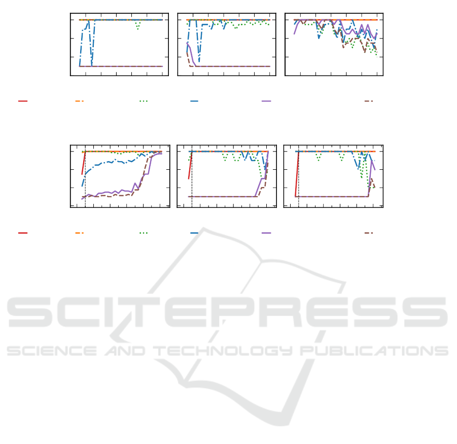
Figure 2: Accuracies of different detection approaches on Synthetic IL-Datasets evaluated using different K for KFCV.

0.0 0.1 0.2 0.3 0.4 0.5

40%

60%

80%

100%

Accuracy

K=10

0.0 0.1 0.2 0.3 0.4 0.5

K=20

0.0 0.1 0.2 0.3 0.4 0.5

K=30

FET-MEAN FET-MEDIAN FET-SUM PTT-MAJORITY PTT-RANDOM (Baseline) DL-LA (Baseline)

Figure 3: Accuracies of different detection approaches on Synthetic IL-Datasets containing datasets with different r.

4.3 Results

In this section, we discuss the results of the experi-

ments outlined above. Recall that K is the number

of folds used for conducting KFCV and r is the pro-

portion of positive instances in the dataset D. Each

IL-Dataset contains binary classiﬁcation datasets of

size 200 ×K. In Figures 2 to 4, we compare the per-

formances (detection accuracy) of FET-MEAN, FET-

MEDIAN, FET-SUM, PTT-MAJORITY with the base-

lines PTT-RANDOM and DL-LA.

Efﬁciency. In Figure 2, the value K (KFCV) is var-

ied between 3 and 30 and shown on the X-axis, and

the resulting accuracy of the ILD approaches along

the Y-axis. Additionally, we compare the perfor-

mance for different choices of class-imbalance pa-

rameter r (r = .1, r = .3, and r = .5 (balanced)), pro-

ducing three individual plots shown side-by-side.

Overall, we observe that the performance of FET-

MEAN and FET-MEDIAN (∼ 100%) does not change

with the value of K (number of estimates) for all three

IL-Datasets, while FET-SUM is very unstable for bal-

anced dataset r = 0.5 and slightly unstable for imbal-

anced datasets. The PTT-MAJORITY approach out-

performs the baselines, but there is no possible ﬁxed

value of K for which the detection accuracy is high re-

gardless of the imbalance. A good choice to prevent

unstable and inaccurate results would require a small

value K < 7 for balanced datasets (r = 0.5) and a

large value K > 7 for imbalanced datasets r = 0.1,0.3,

which is an issue in applications where the imbal-

ance is not known in advance. The reason behind

this could be that Paired T-Test (PTT) produces in-

correct and optimistically biased p-values due to the

low deviation in estimated accuracies of the majority

voting classiﬁer, as explained in the Appendix. An-

other interesting observation is that DL-LA performs

similarly to PTT-RANDOM, which could be because

a Deep multi-layer perceptron can theoretically ap-

proximate any continuous function between input and

output (Cybenko, 1989). Overall, we observed that

Fisher’s Exact Test (FET)-based approaches require a

lower number of estimates K, thus being more efﬁ-

cient in detecting ILs.

Generalization w.r.t. r. In Figure 3, the value r

(class-imbalance) is varied between 0.05 and 0.5 and

shown on the X-axis, and the resulting accuracy of

the ILD approaches along the Y-axis. Additionally,

we compare the performance for different choices of

K (K = 10, K = 20, and K = 30), producing three

individual plots shown side-by-side.

The FET-based approaches perform very well for

all datasets r ≥ 0.05, even if the number of estimates

is as low as K = 10. As before, PTT-MAJORITY

achieves a high detection accuracy for larger numbers

of estimates K = 20,K = 30 only with high imbal-

ance 0.05 ≤ r < 0.3, with deteriorating accuracy for

r ≥ 0.3. The baselines are not able to detect ILs in

imbalanced datasets, as most of the binary classiﬁers

easily achieve an accuracy of 1 −r (same as major-

Automated Information Leakage Detection: A New Method Combining Machine Learning and Hypothesis Testing with an Application to

Side-channel Detection in Cryptographic Protocols

159

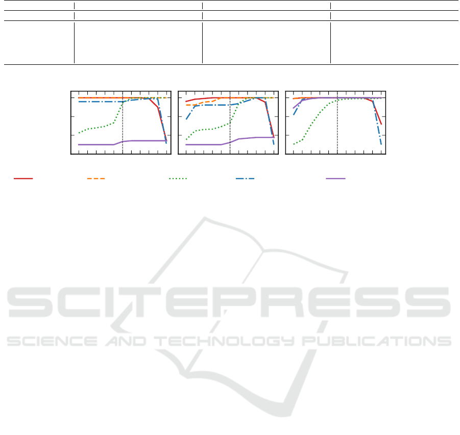
Table 2: Results on the OpenSSL datasets for every approach using K = 20 and m = 1. The best entry is marked in bold.

Class-Imbalance r = 0.1 Class-Imbalance r = 0.3 Class-Imbalance r = 0.5 (Balanced)

Approach FPR FNR ACCURACY F1-SCORE FPR FNR ACCURACY F1-SCORE FPR FNR ACCURACY F1-SCORE

FET-MEAN 0.0021 0.0 0.999 0.999 0.0182 0.0 0.9909 0.9911 0.0164 0.0 0.9918 0.9919

FET-MEDIAN 0.0021 0.0 0.999 0.999 0.0455 0.0 0.9773 0.9778 0.0327 0.0 0.9836 0.9839

FET-SUM 0.66 0.0 0.67 0.7519 0.84 0.0 0.58 0.7043 0.9564 0.0 0.5218 0.6766

PTT-MAJORITY 0.0473 0.0 0.9764 0.9769 0.3309 0.0 0.8345 0.8585 0.3145 0.0 0.8427 0.8674

PTT-RANDOM (Baseline) 1.0 0.0 0.5 0.6667 1.0 0.0 0.5 0.6667 0.1836 0.0 0.9082 0.9179

DL-LA (Baseline) 1.0 0.0 0.5 0.6667 1.0 0.0 0.5 0.6667 0.4727 0.0 0.7636 0.8111

1 2 3 4 5 6 7 8 9 1011

40%

60%

80%

100%

Accuracy

K=20, r = 0.1

1 2 3 4 5 6 7 8 9 1011

K=20, r = 0.3

1 2 3 4 5 6 7 8 9 1011

K=20, r = 0.5 (Balanced)

FET-MEAN FET-MEDIAN FET-SUM PTT-MAJORITY PTT-RANDOM (Baseline)

Figure 4: Accuracies of the detection approaches on OpenSSL Datasets with varying Holm-Bonferroni cut-off parameter m.

ity voting classiﬁer) for them, always outperforming

random guessing (0.5) even when there is no IL.

OpenSSL Dataset. In Table 2, we summarize the

overall performance in terms of FPR, FNR, ACCU-

RACY, and F1-SCORE of ILD approaches on the real

datasets, ﬁxing K = 20 based on the previous re-

sults. Overall FET-MEAN and FET-MEDIAN out-

perform other approaches in detecting side-channel in

the OpenSSL case study. As expected the baselines

work well for balanced datasets while failing to ac-

curately detect side-channels for imbalanced datasets.

The PTT-MAJORITY approach works well for imbal-

anced datasets but produces false positives for bal-

anced datasets. The FET-SUM approach overesti-

mates ILs in the servers, producing false positives for

both balanced and imbalanced datasets.

In Figure 4 we also explore the performance of

ILD approaches for different values of the Holm-

Bonferroni parameter m on these datasets. These re-

sults exclude the DL-LA approach, as it does not use

the Holm-Bonferroni correction. For lower values of

m, some ILD approaches produce a large number of

false positives, because the tests are underestimating

the p-values. Conversely, for larger values of m, the

ILD approaches produce many false negatives, be-

cause not all binary classiﬁers are able to learn an

accurate enough mapping to warrant rejection of the

null hypothesis. Based on the requirements at hand,

it will therefore be necessary to tune m to achieve op-

timal performance. PTT-MAJORITY and FET-SUM

are not reliable for estimating the correct p-values and

produce large false positives, especially for m < 4.

The overall performance of FET-MEDIAN and FET-

MEAN is consistently very high (between 99% and

100%) for all choices of m < 10. FET-MEDIAN is

even more versatile than FET-MEAN, almost always

achieving an accuracy of 100%, because the median

aggregation results in more accurate p-values (Bhat-

tacharya and Habtzghi, 2002).

5 CONCLUSION

We presented a novel machine learning-based frame-

work to detect the possibility of information leak-

age (IL) in a given system. For this, we ﬁrst gener-

ated an appropriate (binary) classiﬁcation dataset us-

ing its observable and secret system data. We then

trained an ensemble of classiﬁcation models using the

dataset. We deduce the existence of IL when either

the ensemble performance is signiﬁcantly better than

majority voting or using the more complex Fisher’s

Exact Test (FET) from statistics.

The major advantages of the presented approach

over previous ones are: (a) it accounts for imbalances

in datasets (b) it has a very low false positive rate (c)

it is robust to noise in the generated dataset (d) it is

time-efﬁcient and still outperforms the state-of-the-

art machine learning-based approaches. These ad-

vantages are partly due to our IL inference using the

non-parametric FET, applied on the confusion ma-

trix of the learning models, rather than direct IL in-

ference using learning accuracies. The robustness,

in particular, is a consequence of using the Holm-

Bonferroni correction technique. We presented exten-

sive empirical evidence for our claims and compared

our approach to other baseline approaches, including

a deep-learning-based one.

In the future, we aim to extend our work to de-

ICAART 2022 - 14th International Conference on Agents and Artiﬁcial Intelligence

160

tect new and unknown side-channels. We are also

interested in exploring IL detection when the gener-

ated dataset yields a multi-class classiﬁcation prob-

lem with ≥ 3 classes. This necessitates extending the

presented FET approach to account for multi-class

classiﬁcation problems. Finally, we would like to

provide appropriate theoretical backing for our ap-

proaches using information theory.

ACKNOWLEDGEMENTS

We would like to thank Bj

orn Haddenhorst, Karlson

Pfanschmidt, Vitalik Melnikov, and the anonymous

reviewers for their valuable and helpful suggestions.

This work is supported by the Bundesministerium f

Bildung und Forschung (BMBF) under the project

16KIS1190 (AutoSCA) and funded by European Re-

search Council (ERC)-802823.

REFERENCES

Bengio, Y. and Grandvalet, Y. (2004). No unbiased estima-

tor of the variance of k-fold cross-validation. Journal

of Machine Learning Research, 5:1089–1105.

Bhattacharya, B. and Habtzghi, D. (2002). Median of the p

value under the alternative hypothesis. The American

Statistician, 56(3):202–206.

Camilli, G. (1995). The relationship between ﬁsher’s exact

test and pearson’s chi-square test: A bayesian perspec-

tive. Psychometrika, 60(2):305–312.

Chatzikokolakis, K., Chothia, T., and Guha, A. (2010). Sta-

tistical measurement of information leakage. In Es-

parza, J. and Majumdar, R., editors, Tools and Algo-

rithms for the Construction and Analysis of Systems,

pages 390–404, Berlin, Heidelberg. Springer Berlin

Heidelberg.

Chicco, D., T

otsch, N., and Jurman, G. (2021). The

matthews correlation coefﬁcient (mcc) is more reli-

able than balanced accuracy, bookmaker informed-

ness, and markedness in two-class confusion matrix

evaluation. BioData Mining, 14(1):13.

Cybenko, G. (1989). Approximation by superpositions of a

sigmoidal function. Mathematics of Control, Signals

and Systems, 2(4):303–314.

Dem

sar, J. (2006). Statistical comparisons of classiﬁers

over multiple data sets. Journal of Machine Learning

Research, 7(1):1–30.

Drees, J. P., Gupta, P., H

ullermeier, E., Jager, T., Konze, A.,

Priesterjahn, C., Ramaswamy, A., and Somorovsky, J.

(2021). Automated detection of side channels in cryp-

tographic protocols: Drown the robots! In Proceed-

ings of the 14th ACM Workshop on Artiﬁcial Intelli-

gence and Security, AISec ’21, page 169–180, New

York, NY, USA. Association for Computing Machin-

ery.

Fisher, R. A. (1922). On the interpretation of χ

from con-

tingency tables, and the calculation of P. Journal of

the Royal Statistical Society, 85(1):87–94.

Geurts, P., Ernst, D., and Wehenkel, L. (2006). Extremely

randomized trees. Machine learning, 63(1):3–42.

Hashemi, M. and Karimi, H. (2018). Weighted machine

learning. Statistics, Optimization and Information

Computing, 6(4):497–525.

Head, T., Kumar, M., Nahrstaedt, H., Louppe, G.,

and Shcherbatyi, I. (2021). scikit-optimize/scikit-

optimize.

Hettwer, B., Gehrer, S., and G

uneysu, T. (2020). Applica-

tions of machine learning techniques in side-channel

attacks: a survey. Journal of Cryptographic Engineer-

ing, 10(2):135–162.

Holm, S. (1979). A simple sequentially rejective multi-

ple test procedure. Scandinavian Journal of Statistics,

6(2):65–70.

ıma, V., Pokorn

y, O., and Rosa, T. (2003). Attacking

rsa-based sessions in ssl/tls. In Walter, C. D., Koc¸,

C¸ . K., and Paar, C., editors, Cryptographic Hardware

and Embedded Systems - CHES 2003, pages 426–440,

Berlin, Heidelberg. Springer Berlin Heidelberg.

Kotsiantis, S. B., Zaharakis, I. D., and Pintelas, P. E.

(2006). Machine learning: a review of classiﬁcation

and combining techniques. Artiﬁcial Intelligence Re-

view, 26(3):159–190.

Koyejo, O., Ravikumar, P., Natarajan, N., and Dhillon,

I. S. (2015). Consistent multilabel classiﬁcation. In

Proceedings of the 28th International Conference on

Neural Information Processing Systems - Volume 2,

NIPS’15, page 3321–3329, Cambridge, MA, USA.

MIT Press.

Moos, T., Wegener, F., and Moradi, A. (2021). DL-

LA: Deep Learning Leakage Assessment: A mod-

ern roadmap for SCA evaluations. IACR Transactions

on Cryptographic Hardware and Embedded Systems,

2021(3):552–598.

Mushtaq, M., Akram, A., Bhatti, M. K., Chaudhry, M.,

Lapotre, V., and Gogniat, G. (2018). Nights-watch:

A cache-based side-channel intrusion detector using

hardware performance counters. In Proceedings of the

7th International Workshop on Hardware and Archi-

tectural Support for Security and Privacy, HASP ’18,

New York, NY, USA. Association for Computing Ma-

chinery.

Nadeau, C. and Bengio, Y. (2003). Inference for the gener-

alization error. Machine Learning, 52(3):239–281.

Pedregosa, F., Varoquaux, G., Gramfort, A., Michel, V.,

Thirion, B., Grisel, O., Blondel, M., Prettenhofer, P.,

Weiss, R., et al. (2011). Scikit-learn: Machine learn-

ing in Python. Journal of Machine Learning Research,

12:2825–2830.

Perianin, T., Carr

e, S., Dyseryn, V., Facon, A., and Guilley,

S. (2021). End-to-end automated cache-timing attack

driven by machine learning. Journal of Cryptographic

Engineering, 11(2):135–146.

Picek, S., Heuser, A., Jovic, A., Bhasin, S., and Regazzoni,

F. (2018). The curse of class imbalance and conﬂicting

Automated Information Leakage Detection: A New Method Combining Machine Learning and Hypothesis Testing with an Application to

Side-channel Detection in Cryptographic Protocols

161

metrics with machine learning for side-channel eval-

uations. IACR Transactions on Cryptographic Hard-

ware and Embedded Systems, 2019:209–237.

Powers, D. M. (2011). Evaluation: From precision, recall

and f-measure to roc., informedness, markedness &

correlation. Journal of Machine Learning Technolo-

gies, 2(1):37–63.

Virtanen, P., Gommers, R., Oliphant, T. E., Haberland, M.,

Reddy, T., Cournapeau, D., Burovski, E., Peterson, P.,

Weckesser, W., et al. (2020). Scipy 1.0: fundamental

algorithms for scientiﬁc computing in python. Nature

Methods, 17(3):261–272.

Zhang, J., Zheng, M., Nan, J., Hu, H., and Yu, N. (2020). A

novel evaluation metric for deep learning-based side

channel analysis and its extended application to im-

balanced data. IACR Transactions on Cryptographic

Hardware and Embedded Systems, 2020(3):73–96.

APPENDIX

Preliminaries

In this section, we formally describe the binary clas-

siﬁcation problem and evaluation metrics. Using

this, we formalize the problem of information leak-

age (IL) in Section 2. Note that, we use these nota-

tions throughout the paper.

Binary Classiﬁcation: Notation and Terminology

In binary classiﬁcation, the learning algorithm is pro-

vided with a set of training data D = {(x

)}

i=0

⊂

X × Y of size N ∈ N, where X = R

is the in-

stance (input) space and Y = {0, 1} the (binary) out-

put space. The task of the learner is to induce a hy-

pothesis h ∈ H with low generalization error (risk)

R(h) =

X ×Y

L(y, h(x))d P(x,y) (4)

where H is the underlying hypothesis space (set of

candidate functions the learner can choose from), L :

Y ×Y → R a loss function, and P a joint probabil-

ity measure modeling the underlying data-generating

process. A loss function commonly used in binary

classiﬁcation is the 0-1 loss deﬁned as L

(y, ˆy) :=

Jy ̸= ˆyK, where JcK is the indicator function returning

a value 1 if condition c is true and 0 otherwise.

The measure P in (4) induces marginal probability

(density) functions on X and Y as well a conditional

probability of the class y given an instance x, so that

we can write p(x,y) = p(y|x) × p(x). Of course,

these probabilities are not known to the learner, so

that (4) cannot be minimized directly. Instead, learn-

ing is commonly accomplished by minimizing (a reg-

ularized version of) the empirical risk

emp

(h) =

∑

i=1

L(y

,h(x

)). (5)

In the following, we denote by ˆg ∈ H an empirical

risk-minimizer, i.e., a minimizer of (5).

Evaluation Metrics

We deﬁne evaluation measures used for binary clas-

siﬁcation as per Koyejo et al. (2015). For a given

D = {(x

)}

i=0

, let y be the ground-truth labels and

ˆy = ( ˆy

,... , ˆy

) predictions, such that ˆy

= ˆg(x

),∀i ∈

[N] := {1,.. .,N}.

Accuracy is deﬁned as the proportion of correct pre-

dictions:

ACC

( ˆy,y) :=

∑

i=0

J ˆy = yK.

Confusion Matrix. Many evaluation metrics is de-

ﬁned using true positive (TP), true negative (TN),

false positive (FP) and false negative (FN). Formally,

they are deﬁned as: TN( ˆy, y) =

∑

i=0

= 0, ˆy

0K,TP( ˆy,y) =

∑

i=0

= 1, ˆy

= 1K,FP( ˆy, y) =

∑

i=0

= 0, ˆy

= 1K,FN( ˆy, y) =

∑

i=0

= 1, ˆy

= 0K.

Using these, the Confusion Matrix is deﬁned as:

( ˆy,y) =



TN( ˆy,y) FP( ˆy,y)

FN( ˆy,y) T P( ˆy,y)



F1-Score. F1-SCORE is an accuracy measure which

penalizes the FP more than FN and deﬁned as:

( ˆy,y) =

2TP( ˆy,y)

(2TP( ˆy,y)+FN( ˆy,y)+FP( ˆy,y))

False Negative Rate. FNR is deﬁned as the ratio of

FN to the total positive instances:

FNR

( ˆy,y) =

FN( ˆy,y)

(FN( ˆy,y)+T P( ˆy,y))

False Positive Rate. FPR is deﬁned as the ratio of

FP to the total negative instances:

FPR

( ˆy,y) =

FP( ˆy,y)

(FP( ˆy,y)+T N( ˆy,y))

Statistical Tests

In this section, we explain the statistical tests in more

detail, which are used for our proposed information

leakage detection (ILD) approaches in Section 3.

Paired T-Test (PTT)

PTT is used to compare two samples (generated from

an underlying population) in which the observations

in one sample can be paired with observations in

ICAART 2022 - 14th International Conference on Agents and Artiﬁcial Intelligence

162

the other sample (Dem

sar, 2006). We apply K-Fold

cross-validation (KFCV) and use the same K train-

test datasets pairs for evaluating the majority voting

classiﬁer and binary classiﬁers, to produce K paired

accuracy estimates of majority voting classiﬁer (a

)

with the binary classiﬁer (a

). For binary classi-

ﬁer C

, let H

= a

) be the null hypothesis and

̸= a

) be the alternate hypothesis. H

) indicates that the underlying distribution of two

populations is the same, which means that there is no

difference between the performance of 2 binary clas-

siﬁers (Dem

sar, 2006). H

̸= a

) instead implies

that there is a signiﬁcant difference between the per-

formance of 2 binary classiﬁers.

The p-value quantiﬁes the probability of accept-

ing H

and is evaluated by determining the area un-

der the Student’s t-distribution curve at value t, which

is 1 −cdf(t). The t-statistic is evaluated as t =

√

such that µ =

∑

k=1

, d

= a

−a

mck

and σ

∑

k=1

(µ−d

)

K−1

. Nadeau and Bengio (2003) pro-

posed to adjust the variance for considering the de-

pendency in estimates due to KFCV is deﬁned as

Cor

= σ(

K−1

). This variance σ

Cor

is used to cal-

culate value of t-statistic as t =

Cor

. PTT requires a

large number of estimates (large K) to produce a pre-

cise p-value, which diminishes the effect of the cor-

rection term

(K−1)

for σ

Cor

and produces imprecise

accuracy estimates as the test set size reduces.

Fisher’s Exact Test (FET)

FET is a non-parametric test which is used to calcu-

late the probability of signiﬁcance independence (non

dependence) between two classiﬁcations methods by

analyzing the contingency table containing the result

of classifying objects by two methods (Fisher, 1922).

For example, given a sample of people, we can divide

them based on gender and based on if they like cricket

as a sport. Assuming that the sample is a good repre-

sentation of people and, for the sake of argument, gen-

erally most of the men in our sample like cricket, and

most of the women do not. The FET would produce a

very low p-value, implying that the two classiﬁcation

methods are correlated.

The p-value is computed using Hypergeometric

distribution as:

Pr(M)(N,R, r) =

(R)

(TN)

×C

(N−R)

(r−TN)

(N)

(r)

(FN+TN)

(TN)

×C

(FP+T P)

(FP)

(TP+TN+FP+FN)

(TN+FP)

where r = TN + FP, N = FP+ TP+ FN + TN, R =

TN + FN and C

(n)

(r)

is the combinations of choosing r

items from the given n items. The p-value is calcu-

lated by summing up the probabilities Pr(M) for all

tables having a probability equal to or smaller than

that observed M. This test considers all possible ta-

bles with the observed marginal counts for TN of the

matrix M, to calculate the chance of getting a table at

least as “extreme”. P-value for majority voting classi-

ﬁer using above equation is Pr(X = TN) = 1.0, as if

the predicted class is 0 ( ˆy = 0), then FP = 0,TP = 0

and if it is 1 ( ˆy = 1), then FN = 0, TN = 0.

Relation to Mathews Correlation Coefﬁcient.

Mathews Correlation Coefﬁcient (m

MCC

) is a bal-

anced accuracy evaluation measure that penalizes FP

and FN equally and accounts for imbalance in the

dataset (Chicco et al., 2021). Camilli (1995) showed

that, m

MCC

is directly proportional to the square root

of the χ

statistic, i.e., |m

MCC

| =

/N and the χ

statistical test is asymptotically equivalent to FET.

For majority voting classiﬁer and random guessing

MCC

= 0, thus χ

= 0, producing the χ

p-value

as 1 (Camilli, 1995). This indirect relation to Math-

ews Correlation Coefﬁcient makes FET an appropri-

ate statistical test for testing the learnability of a bi-

nary classiﬁer using the confusion-matrix while tak-

ing imbalance in the dataset into account.

Holm-Bonferroni Correction

The Holm–Bonferroni method controls the family-

wise error rate (probability of false positive or Type

1 errors) by adjusting the rejection criteria α for each

individual hypotheses (Holm, 1979). We consider a

family of null hypotheses F = H

,... , H

and ob-

tain p-values p

,... , p

, from independently testing

each classiﬁer C

∈ C , such that J = |C | For getting

an aggregated decision, the signiﬁcance level for the

set F is not higher than the pre-speciﬁed threshold

α = 0.01. The p-values are sorted in ascending or-

der, i.e. p

≤ p

,... p

j−1

≤ p

, and for each hy-

pothesis H

∈ F , if p

J+1−j

, H

is rejected. Let

m+1

be ﬁrst hypothesis for which the p-value does

not validate rejection, i.e. p

m+1

J−m

. Then, the re-

jected hypotheses are {H

,... , H

} and the accepted

hypothesis are {H

m+1

,... , H

IL Detection. We imply that even if one of the

∈ F is rejected, i.e. m >= 1, then IL exists in

the system. This increases the probability of obtain-

ing false positives increases. So, we have also ana-

lyzed the performance of our approaches for different

values of m on real-dataset as described in Section 4.3

Automated Information Leakage Detection: A New Method Combining Machine Learning and Hypothesis Testing with an Application to

Side-channel Detection in Cryptographic Protocols

163