Combining a Grayscale Camera and Spectrometers for High Quality

Close-range Hyperspectral Imaging of Non-planar Surfaces

Stefan L

orcks

and Josef Pauli

Intelligent Systems Group, University of Duisburg-Essen, Germany

Keywords:

Hyperspectral Imaging, Spectroscopy, Surface Analysis, Metrology, Calibration, Depth Map, Dataset.

Abstract:

In recent years, hyperspectral imaging (HSI) has emerged to become a crucial method for both remote sensing

and close-range surface analysis. In this paper, we present substantial upgrades of our previously published

system for multispectral and hyperspectral surface analysis (Hegemann et al., 2017). Besides minor changes

in illumination, we carefully evaluated different approaches for reﬂectance correction using up to eight cal-

ibration standards. Wavelength correction, which ensures an exact wavelength ﬁt, is also done using a cali-

bration standard. Therefore, our calibration pipeline provides high-quality hyperspectral data that is mostly

independent of the hardware acquiring it, as we remove the impact of illumination and sensor sensitivity and

consequently solely dependent on the sample. Additionally, as the main contribution, we present a method to

acquire hyperspectral images from a non-planar surface using spectrometers without a time-consuming auto-

focus at every pixel position. We do this by generating a registered depth map from gray value images of the

sample. Since annotated hyperspectral data is in high demand, we also contribute two initial pixel-wise labeled

close-range hyperspectral datasets generated with our upgraded system for further research and benchmarks.

1 INTRODUCTION

Hyperspectral imaging (HSI) is well established in

remote sensing. With the increasing availability of

portable hyperspectral cameras in recent years, HSI

also became more prevalent in close-range surface

analysis with a wide range of applications (Khan

et al., 2018b). For example, HSI has been used to

estimate the biomass on a ﬁeld (P

onen et al., 2013)

or the damage of beetle infestation in a forest (N

asi

et al., 2015). Furthermore, (Halicek et al., 2020) ex-

amined the impact of HSI for detecting tumors. Ex-

amples of the usage of HSI in the food industry are

listed in (Liu et al., 2017) and (Park and Lu, 2015).

Moreover, (Liang, 2012) shows how HSI is applied in

art analysis.

Hyperspectral imaging adds a spatial dimension

to spectroscopy. A spectrum is acquired at each po-

sition of a grid. Therefore, in a hyperspectral image,

each pixel contains not only one intensity value as in a

grayscale image but hundreds or even thousands of re-

ﬂectance values for different wavelengths. The range

of wavelengths extends the visible light towards both

ultraviolet light as well as infrared light. A hyper-

https://orcid.org/0000-0003-3641-4734

https://orcid.org/0000-0003-0363-6410

spectral image has three dimensions: two spatial di-

mensions and one spectral dimension.

Hyperspectral cameras can acquire images using

different techniques. Commonly used approaches are

snapshot cameras (Hagen and Kudenov, 2013), push

broom (or linescan) cameras (Lu and Fei, 2014) and

whisk broom (or pointscan) cameras (Kerekes and

Schott, 2007). Whisk broom scanners follow a spa-

tial scanning scheme and acquire the full spectrum at

a single position at a time.

As always in metrology, calibration is essential in

hyperspectral imaging to produce useful data. Re-

ﬂectance calibration (reﬂectance correction) is a com-

mon procedure in hyperspectral imaging to reduce

the impact of illumination and sensory equipment in

the data. (Burger and Geladi, 2005) suggested three

different models for the reﬂectance correction: sim-

ple, linear, and quadratic. Whereas the simple ap-

proach uses just one reﬂectance standard, the linear

and quadratic model can take several reﬂectance stan-

dards into account. The simple approach is the com-

monly used, e.g. in (Klein et al., 2008), (Yao and

Lewis, 2010), (Halicek et al., 2020).

When it comes to classifying hyperspectral data,

deep learning approaches are state of the art (Paoletti

et al., 2019), (Rasti et al., 2020). As these are su-

Lörcks, S. and Pauli, J.

Combining a Grayscale Camera and Spectrometers for High Quality Close-range Hyperspectral Imaging of Non-planar Surfaces.

DOI: 10.5220/0010789300003121

In Proceedings of the 10th International Conference on Photonics, Optics and Laser Technology (PHOTOPTICS 2022), pages 26-37

ISBN: 978-989-758-554-8; ISSN: 2184-4364

pervised learning methods, annotated data is essen-

tial for training and evaluation. Unfortunately, only

a few datasets with pixel-wise annotations are pub-

lically available, e.g., ”Indian Pines” (Baumgardner

et al., 2015), ”Salinas”, ”Pavia University”, ”Hous-

ton University”. These datasets all originate from re-

mote sensing. The available close-range datasets are

either not equipped with a pixel-wise ground truth or

provide just a low spectral resolution and range (Pao-

letti et al., 2019). For example, (Khan et al., 2018a)

provides a close-range HSI dataset of different mate-

rials (mainly textile) but just image-wise class labels

and wavelengths between 400 nm and 1,000 nm. To

the best of our knowledge, no pixel-wise annotated

close-range hyperspectral images comparable to the

datasets presented in this paper are publicly available

yet.

This paper is organized as follows: In chapter 2

the preliminary system is summarized. Then, the up-

grades made to the system to provide even better data

are described in chapter 3. Two annotated datasets

acquired with the system and published together with

this paper are presented in the second to last chapter.

The ﬁnal chapter concludes the article and gives an

outlook on future work.

2 PRELIMINARY SYSTEM

Our imaging system consists of a gray value cam-

era and two spectrometers working in a whisk broom

scanning manner. This means that the spectrometers,

which share one objective, acquire a spectrum at one

spatial position (pixel) at a time. A hyperspectral im-

age is generated by scanning the sample such that the

objective is positioned at every pixel position. This is

done using a 3D Cartesian robot. The ﬁrst axis car-

ries the sample (left/right). The measurement head

consisting of the gray value camera and the spec-

trometer head is mounted on a different part of the

Cartesian robot, moving in two directions (up/down,

front/back). These components are shown in ﬁgure 1.

The construction allows moving the sample and

objectives (of the camera and the spectrometers) to

acquire a hyperspectral image or a grayscale image

of the sample. Furthermore, the grayscale camera

and the spectrometer head are geometrically cali-

brated towards each other using a 2D calibration pat-

tern (Hegemann et al., 2017). This means their 3D-

translation and 2D-rotation are known. Therefore, a

part of the sample acquired with the camera can be

acquired with the spectrometer head easily by mov-

ing the robot axes the corresponding distances.

The grayscale camera used is the Baumer SXG80.

It provides a resolution of 3296 × 2472 pixels. The

Qioptiq inspect.x L objective is ﬁxed. Focusing can be

done by adjusting the distance between the sample’s

surface and the camera (by moving the camera up and

down). The objective leads to a real-world pixel size

of 3.57 µm × 3.57 µm.

The two spectrometers used are the BaySpec Su-

per Gumet UV-NIR spectrometer (190 nm - 1,100 nm)

and the BaySpec Super Gamut NIR (900 nm - 1,700

nm). For better readability, we will denote the spec-

trometers as UV-NIR and NIR, respectively. They

are coupled to one Nikon TU Plan Fluor 10x objec-

tive using a dichroic mirror reﬂecting the light below

950 nm towards the UV-NIR spectrometer and light

above 950 nm towards the NIR spectrometer via op-

tical ﬁbers. The ﬁeld of view of the objective both

spectrometers share is a disc with a diameter of about

60 µm. The spectral resolution of the two spectrome-

ters differs as the UV-NIR provides 3648 bands with

a spectral resolution of 0.254 nm, whereas the NIR

spectrometer has a lower spatial resolution of 3.219

nm as it provides 256 bands. The distance between

the spectrometer head and sample (provided by the Z-

axis) has been determined using the geometrical cali-

bration.

The auto-focus of the spectrometer head is very

time-consuming. Therefore, an auto-focus is done us-

ing the grayscale camera. Afterwards, the spectrome-

ter head can be brought into the in-focus height using

the calibration between the objectives. This is suf-

ﬁcient for a planar sample, where the whole sample

can be acquired at the same height. Unfortunately,

non-planar samples, where every pixel position needs

a different height to be in the focus of the spectrome-

ter head, are more challenging. A method to acquire

height adaptive hyperspectral images for non-planar

samples is presented in the next section, which sum-

marizes the improvements made to the system.

3 ADVANCED SYSTEM

The above described preliminary system has been up-

graded to provide hyperspectral images of better qual-

ity and from a broader range of samples. Therefore,

several changes in both hardware and software have

been made. The following section 3.1 describes how

the hardware has been changed to provide more dif-

fuse illumination. In section 3.2 the post-processing

of the raw data provided by the spectrometers into cal-

ibrated reﬂectance data is speciﬁed. A procedure to

acquire hyperspectral data from non-planar samples

is introduced in section 3.3. Finally, the possible ac-

quisition modes of the system are summarized in 3.4.

Combining a Grayscale Camera and Spectrometers for High Quality Close-range Hyperspectral Imaging of Non-planar Surfaces

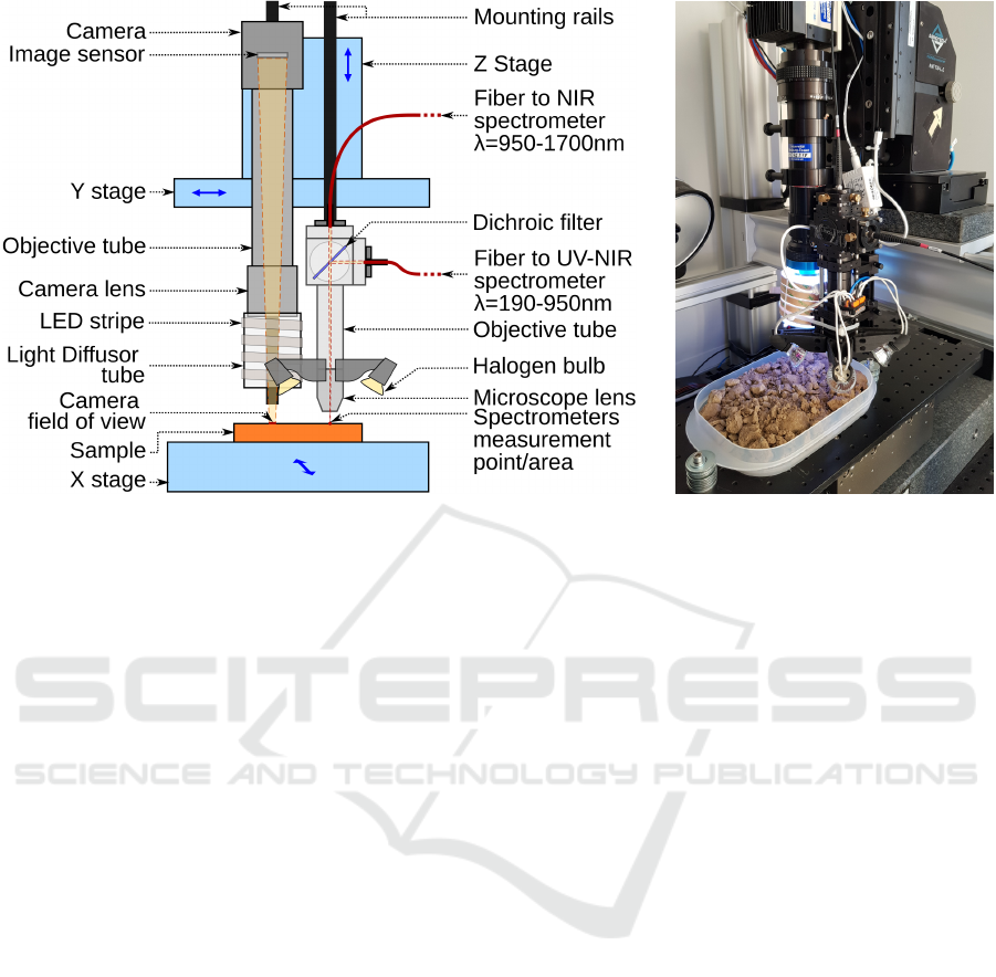
(a) Schematic of the measurement head and the axes. (b) Actual system inspecting soil.

Figure 1: The measurement head consists of the grayscale camera and their objective as well as the spectrometer head (both

equipped with illumination). Those are mounted to the Z-axis of the Cartesian robot which in turn is mounted to the Y-axis.

The sample is carried by the X-axis as can be seen in the schematic in (a) (Adapted from (Hegemann et al., 2017)). An image

of the actual system can be seen in (b).

3.1 Illumination Upgrades

In the preliminary system design, a low-cost, high

voltage halogen lamp has been used for one-

directional illumination underneath the spectrometer

head. This design has been suitable for planar sample

surfaces. For non-planar samples, though, illumina-

tion from just one side could lead to massive shad-

owing and, consequently, a low signal-to-noise ratio.

We, therefore, upgraded the illumination design for

the spectrometers by mounting custom-designed 3D

printed halogen bulb holders to the spectrometer head

(see ﬁgure 1). This means the sample under the lens

center is now illuminated from four directions with 90

degrees between the lamps. This ensures that the sam-

ple is still brightly illuminated even if the non-planar

surface of the sample blocks some light.

The illumination for the grayscale camera has

been upgraded as well. Beforehand, ﬁve different

LED lamps (”white”, red, green, blue, IR) mounted

in different positions have been used. Naturally, they

illuminated the sample from different angles leading

to different shadows on non-planar surfaces. Also,

gloss reﬂections have been an issue with shiny sur-

faces (such as metal) as the used diffusor did not have

the expected impact. We improved this by coiling a

LED stripe directly around the diffusor. The solution

provides a very diffuse light from all directions.

3.2 Postprocessing of the Measured

Data

Two post-processing steps are applied on the data pro-

vided by the spectrometers: reﬂectance correction and

wavelength correction. Why they are needed and how

we use them is described in detail in this section.

3.2.1 Reﬂectance Correction

The raw measurements a spectrometer delivers are

so-called digital numbers (DN). Their range depends

on the analog-to-digital converter in the spectrome-

ter. The digital number for a speciﬁc wavelength de-

pends on the illumination (amount of photons of this

wavelength emitted by the source), on the reﬂectance

(amount of the incoming photons of this wavelength

reﬂected by the sample), and the sensitivity of the sen-

sor (quantum efﬁciency for this wavelength). Usually,

one is interested in the characteristic of the sample

and not so much in the illumination or the sensor’s

sensitivity. Therefore, we use reﬂectance correction

approaches to estimate the sample reﬂectance based

on the measured digital numbers.

Let λ be the wavelength in nanometers. The dig-

ital numbers and the reﬂectance for a speciﬁc wave-

length are denoted by DN(λ) and R(λ), respectively.

The dark current, which is the sensor’s output with-

out illumination, depends on the wavelength λ as

PHOTOPTICS 2022 - 10th International Conference on Photonics, Optics and Laser Technology

well. Therefore, we denote it as D(λ). If for at

least one object the reﬂectance R(λ) would be known

(and the digital numbers DN(λ) have been measured),

one would have pairs of corresponding values R(λ)

and DN(λ) for each wavelength. Such objects with

a known reﬂectance are called reﬂectance standards.

For a reﬂectance standard the reﬂectance R

(λ) is

known. Using this one reﬂectance standard as the

sample, we measure the digital numbers DN

(λ).

For the reﬂectance correction (Klein et al., 2008)

suggest

R(λ) = R

(λ) ·

DN(λ)− D(λ)

(λ) − D(λ)

, (1)

which allows us to calculate the reﬂectance of a sam-

ple for every wavelength, given the digital numbers

of the sample, the dark current, the digital numbers of

the reﬂectance standard and the reﬂectance of the re-

ﬂectance standard. This is what (Burger and Geladi,

2005) call the simple model. Here, only one re-

ﬂectance standard is required besides the dark cur-

rent. Typically, a ”white” standard is used, which re-

ﬂects all wavelengths almost completely. (Burger and

Geladi, 2005) also suggest

R(λ) = b

(λ) · DN(λ) + b

(λ), (2)

and

R(λ) = b

(λ) · DN(λ)

+ b

(λ) · DN(λ) + b

(λ),

(3)

which they call the linear model and quad(ratic)

model, respectively. Here, the reﬂectance is inter-

preted as a polynomial function of the digital num-

bers. The coefﬁcients b

(λ), b

(λ) and possibly b

(λ)

are estimated using several reﬂectance standards and

least-squares regression. The dark current can be used

as well but unlike in the simple model it is not re-

quired. Based on these proposals, we formulate a cu-

bic model

R(λ) =b

(λ) · DN(λ)

+ b

(λ) · DN(λ)

+ b

(λ) · DN(λ) + b

(λ). (4)

We evaluated all four models (eq. 1: simple

model, eq. 2 linear model, eq. 3: quadratic model,eq.

4: cubic model) by means of the following steps:

1. Measurement of the digital numbers of the dark

current and eight Zenith Polymer

reﬂectance

standards by SphereOptics.

2. Calculation of the coefﬁcients of all wavelengths

for all four models based on (subsets of) these

measurements.

3. Application of the models to the measurements

and evaluation of the estimated reﬂectances, both

quantitative and qualitative.

These steps are described in detail in the following

paragraphs.

Measurements. The standards have the nominal re-

ﬂectances 99 %, 80 %, 60 %, 50 %, 25 %, 10 %, 5

% and 2.5 %. The exact wavelength-dependent re-

ﬂectance values R

(λ) are provided with the stan-

dards. The Zenith Polymer

reﬂectance standards

have non-homogeneous surfaces. They consist of

brighter and darker parts, whose ratio is such that

the surfaces have the aspired reﬂectance on average.

Because of this spatial divergence, it is necessary to

acquire a surface patch and not just one position.

We use 62,500 measurements over an area of about

15 mm × 15 mm. These measurements are averaged

to reduce the noise and come up with digital numbers

of the reﬂectance standards DN

(λ). They are visual-

ized in ﬁgure 2a.

One can see the decrease in digital numbers from

the 99 % standard to the 2.5 % standard for each

wavelength. It is also obvious why reﬂectance cor-

rection is necessary: If the illumination and the spec-

trometer sensitivity were wavelength-independent,

the digital numbers should form a horizontal line for

each standard, which is not the case. One can also see

the difference in spectral resolution between the spec-

trometers. While the measurements of the UV-NIR

spectrometer almost appear as a continuous line, the

data produced by the NIR spectrometer is discrete and

has a lower spectral resolution. Another effect that

can be seen here is the dichroic mirror which leads to

lower digital numbers around 950 nm and therefore a

lower signal-to-noise ratio. Additionally to the eight

reﬂectance standards also the dark current has been

measured.

Calculations. For calculating the coefﬁcients of the

models, we used different subsets of the measure-

ments. For the simple model (eq. 1), just the measure-

ments of the standard with the highest reﬂectance and

the dark current are used. The simple model has two

variants: The ﬁrst (”simple100”) assumes the stan-

dard to be fully reﬂective for all wavelengths, which

leads to R

(λ) = 1 for all wavelengths. The sec-

ond variant (”simple99”) takes the actual reﬂectance

of the standard into account. For the linear, the

quadratic, and the cubic model, we calculate two

variants each: Based on the eight reﬂectance stan-

dards (”linear8”, ”quad8” and ”cubic8”) as well as

on the eight standards and the dark current (”linear9”,

”quad9” and ”cubic9”). Here, the coefﬁcients are de-

termined using a least-squares polynomial ﬁtting.

Evaluation. After calculating the coefﬁcients for all

model variants, we evaluated the variants on the mea-

surements of the reﬂectance standards and the dark

current. The models have been applied to all 62,500

Combining a Grayscale Camera and Spectrometers for High Quality Close-range Hyperspectral Imaging of Non-planar Surfaces

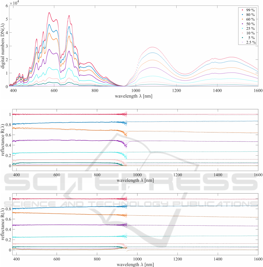
(a) Before reﬂectance correction: Spatially averaged digital numbers after dark current subtraction.

(b) After reﬂectance correction using the ”simple100” model.

Figure 2: The average digital numbers (a) are far from the ideal horizontal lines for all standards. The reﬂectance correction

results for ”simple100” model (b) and ”cubic8” model (c) both show a clear improvement to the digital numbers. The gray

dashed lines show the true reﬂectance values of the standards, while the colored dots show the results of the reﬂectance

correction. The colors correspond to the digital numbers in (a).

positions, and afterwards, the median reﬂectance has

been determined. These median values have then

been compared to the actual reﬂectance values by

calculating the mean absolute error (MAE) over all

wavelengths. Table 1 lists the errors for all model

variants and all standards, as well as the dark current,

denoted as ”0 %”. Additionally, for each model vari-

ant, the average over the MAEs of all standards has

been determined. As the values are relatively small,

they are given per thousand (‰). The common ”sim-

ple100” model has the worst results. They can be im-

proved by using the standard’s real reﬂectance val-

ues, which is done in ”simple99”. The polynomial

regressions result in even lower average errors. The

usage of the dark current on top of the reﬂectance

standards deteriorates the results. The best effect can

be achieved using the ”cubic8” model. The median

reﬂectances of the ”simple100” model are shown in

PHOTOPTICS 2022 - 10th International Conference on Photonics, Optics and Laser Technology

ﬁgure 2b. The model systematically overestimates the

reﬂectance for the brighter standards (99 %, 80 %, 60

%, and 50 %). For all standards, there are two prob-

lematic wavelengths areas. The ﬁrst is around 400

nm, where the given illumination is too low. The sec-

ond is the area around 950 nm, where the sensitivity

of the spectrometers is relatively low and the dichroic

mirror decreases the signal as well.

Figure 2c, presenting the reﬂectance correction

results using the best-performing ”cubic8” model,

shows an improvement for most standards and the

dark current compared to the ”simple100” model.

3.2.2 Wavelength Correction

By doing the reﬂectance correction, we calibrated the

ordinate of our reﬂectance data (vertical alignment).

However, one can also calibrate the abscissa. This

corresponds to the question: Does the digital num-

ber, which the spectrometer provides for some wave-

length λ

, belong to this exact wavelength or maybe

to a slightly higher or lower wavelength λ? We use a

Zenith Polymer

wavelength standard by SphereOp-

tics, which is enriched with rare-earth oxides. This

leads to sharp peaks in the reﬂectance curve at known

wavelengths. Acquiring an image of the reﬂectance

standards allows adjusting the measured peaks to the

known wavelengths.

The reﬂectance of the wavelength standard-based

measurements by both spectrometers as well as the

true reﬂectance of the standard is shown in ﬁgure 3a

- The peaks of the NIR spectrometer reﬂectance and

the true reﬂectance match. However, the reﬂectance

acquired by the UV-NIR spectrometer shows a clear

mismatch. The provided wavelengths are too high and

need to be adjusted.

The model used for wavelength adaption is a sec-

ond degree polynomial (quadratic function):

λ(λ

) = a

· λ

+ a

· λ

+ a

To ﬁnd optimal values for the coefﬁcients a

, a

polynomial regression is done based on correspond-

ing pairs of (manually selected) peaks (10 for the UV-

NIR spectrometer, 5 for the NIR spectrometer).

The resulting reﬂectances after applying the wave-

length correction are visualized in ﬁgure 3b. Notice-

ably, the peaks in the range of the UV-NIR spectrom-

eter match signiﬁcantly better than without the wave-

length correction.

3.2.3 Overall Postprocessing

For the reﬂectance correction to work correctly, it is

necessary to have the wavelengths corrected. Other-

wise, the wrong reﬂectance values are used for esti-

mating the model. However, for the wavelength cali-

bration, it is required to have reﬂectance values. This

problem is solved by a three-step procedure. First,

a reﬂectance correction is done. The resulting re-

ﬂectance curves are used in a second step to deter-

mine the peak positions and perform the wavelength

correction. As just the peak position on the wave-

length axis is important here, it is neglectable that

the height does not ﬁt exactly. On the now matching

wavelengths, the reﬂectance correction can be done

as the third and ﬁnal step. Once the coefﬁcients for

wavelength and reﬂectance correction are determined,

they can be used to convert the digital numbers from

a sample into reﬂectance values, which are only de-

pendent on the sample.

3.3 Height Adaptive Spectroscopy for

Non-planar Samples

The acquisition of hyperspectral images from planar

samples has been possible with our system in the

past. This has been sufﬁcient as the system was built

for surface inspection of steel plates (Herwig et al.,

2012). However, to be able to examine a wider variety

of samples (namely those with a non-planar surface),

we decided to upgrade the system accordingly.

Acquiring images from non-planar samples is

easy for cameras with a broad depth of ﬁeld. How-

ever, for a spectrometer-based whisk broom solution

with a narrow depth of ﬁeld, acquiring data from non-

planar samples is difﬁcult. The naive way is to do an

autofocus procedure with the spectrometer at every

pixel position. Yet, this is very time-consuming as for

every pixel position the hyperspectral image has to be

acquired in all possible heights.

Instead, we propose a procedure making use of

the grayscale camera, which can acquire an area in-

stead of just one position. We use the grayscale cam-

era to estimate the height of the sample at every point.

Knowing the height, the spectrometer head can be po-

sitioned accordingly and the spectra can be acquired

in focus for a non-planar sample.

The grayscale camera’s objective is tuned to pro-

vide a narrow depth of ﬁeld. This means, for a part of

the image to be in focus, the range of heights is very

small. Figure 4 shows the Brenner focus measure (eq.

5) for different heights. The full width at half maxi-

mum (FWHM) is about 0.31 mm. The same holds for

the spectrometer head (FWHM of UV-NIR: 1.4 mm,

FWHM of NIR: 1.2 mm) as shown in ﬁgure 4. Based

on the geometric calibration, the offset between the

focus heights of the grayscale camera and spectrom-

eter is known (Hegemann et al., 2017). Therefore,

if the focus heights of the whole sample are known

Combining a Grayscale Camera and Spectrometers for High Quality Close-range Hyperspectral Imaging of Non-planar Surfaces

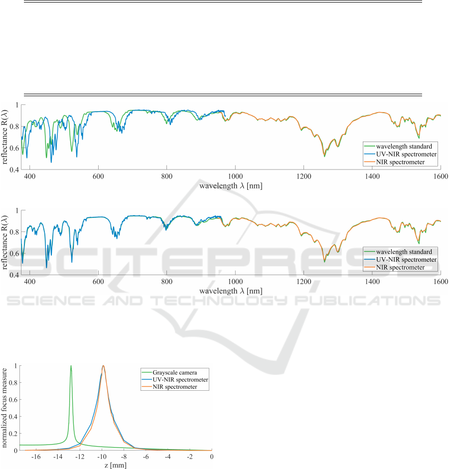
Table 1: The reﬂectance correction model variants are applied to the 62,500 measurements of each reﬂectance standard and

dark current and the median reﬂectance is determined. For all variants, the mean absolute error between median reﬂectance

and true reﬂectance is listed for every standard, the dark current, and in average. All values are per thousand (‰).

Model variant 99 % 80 % 60 % 50% 25% 10% 5% 2.5% 0% Average

simple100 8.39 4.60 12.44 9.62 5.40 8.16 9.04 8.70 0.06 7.38

simple99 1.62 4.83 8.88 7.97 6.20 9.06 9.46 8.86 0.06 6.33

linear8 4.06 4.94 6.22 5.59 2.14 2.38 2.11 3.15 8.14 4.30

linear9 4.12 4.81 6.27 5.56 2.29 3.54 3.47 3.79 6.27 4.46

quad8 2.22 5.11 3.96 1.91 2.45 2.67 1.55 1.54 10.10 3.50

quad9 1.90 4.85 4.57 2.37 2.69 4.16 3.60 2.43 6.85 3.71

cubic8 2.24 5.04 3.78 1.92 2.12 2.61 1.72 1.00 9.90 3.37

cubic9 2.58 5.70 3.44 2.49 1.74 3.46 3.80 3.12 5.74 3.56

(a) Before wavelength correction.

(b) After wavelength correction.

Figure 3: The reﬂectance of the wavelength standard shows several sharp peaks due to the rare-earth oxides. These peaks

are used to calibrate the wavelength axis. The true reﬂectance of the standard as well as the reﬂectance acquired by both

spectrometers (UV-NIR and NIR) before the wavelength correction are visualized. The UV-NIR spectrometer has a large

offset before the correction (a) which is diminished after the correction (b).

Figure 4: Focal stacks have been acquired with the

grayscale camera and both spectrometers for a plane sam-

ple. The normalized Brenner focus measure has been cal-

culated for all heights for all three sensors. The three curves

show a clear and sharp peak which corresponds to the nar-

row depth of ﬁeld of the objectives. Because of the narrow

depth of ﬁeld of the camera, the height can be estimated

based on the focus measure.

for the grayscale camera, which is relatively easy to

achieve, the focus heights for the spectrometer head

are known just by adding the offset. The focus heights

can be thought of as a depth map as well. The follow-

ing section describes how it is generated.

3.3.1 Depth Map Generation

The depth map modeling the surface height of the

sample is generated out of a focal stack (a stack of

pictures taken at different heights) produced by the

grayscale camera. The focal stack consists of images

where z denotes the height at which the images

have been taken. The z-axis provides values between

−17.5 mm and 17.5 mm. For the focal stack, we use

a step size of 0.1 mm. This means a focal stack can

contain up to 351 images.

On every image in the focal stack, a focus mea-

sure is applied. A focus measure takes an image as

PHOTOPTICS 2022 - 10th International Conference on Photonics, Optics and Laser Technology

input and returns a value for every pixel describing

how much this pixel is in focus. A wide variety of

focus measures is available (Pertuz et al., 2013). As

a trade-off between accuracy and time consumption,

we use a variation of the Brenner focus measure to

come up with a value for every pixel position (i, j):

(i, j) =| f

(i, j) − f

(i + 2, j)|

+ | f

(i, j) − f

(i, j + 2)| (5)

The resulting pixel-wise focus measure FM

is af-

terwards averaged on blocks of 56 px × 56 px (≈

0.2 mm×0.2 mm) leading to the mean focus measure

FM with a lower spatial resolution.

This spatial resolution is sufﬁcient for the depth

map but avoids unnecessary computational cost. The

depth map is generated by evaluating at which height

the focus measure reaches its maximum for every

block (k, l):

DM(k, l) = argmax



(k, l)



Similarly, an all-in-focus image can be extracted out

of the focal stack. Figure 5 shows an example. Three

gray value images out of the focal stack are shown in

(a)-(c) and the corresponding mean focus measures in

(e)-(g). The all-in-focus image is shown in (d), the

resulting depth map is visualized in (h).

Using the geometrical calibration, the average x

and y world coordinates for each entry of the depth

map are determined. The value of the depth map is

the z world coordinate.

3.3.2 Height Adaptive HSI

The described depth map generation is done for every

focal stack. The focal stacks have a slight overlap and

cover the whole sample. The resulting world coor-

dinates are combined into a single three-dimensional

point cloud. Because of the construction of the sys-

tem, the camera and the spectrometer head have a

different ﬁeld of view (FOV). Their FOVs have an

overlapping area, whose width is 3 cm. To be able

to acquire data from larger samples, we ﬁrst place the

sample in the FOV of the camera to come up with

the depth map. Afterwards, the sample is placed in

the spectrometer FOV and partly in the overlapping

area. Another smaller depth map is generated in the

overlapping area. The resulting point clouds are reg-

istered using the iterative closest point (ICP) algo-

rithm to come up with the sample height mapped to

the position in the spectrometer FOV. For all (x, y)

coordinates where the spectrum should be acquired,

the height is estimated out of the point cloud us-

ing nearest-neighbor interpolation. The spectrometer

head is then moved to the corresponding position and

measurements are taken in focus.

Figure 6 shows an example of the improvement of

the adaptive height HSI measurements for non-planar

samples. A stack of coins has been used as a non-

planar sample. It is shown in ﬁgure 6a. Two hy-

perspectral images of the sample have been acquired:

One at a ﬁxed height (as so far used for planar sam-

ples) and one at adapted heights based on the before-

hand explained procedure. To visualize the differ-

ences between the two hypercubes, pseudo RGB im-

ages have been created out of them. The ﬁxed height

hyperspectral image is in focus for the second-highest

coin. However, parts of the sample, which are lower

or higher, are blurry. In contrast, in the height adap-

tive hyperspectral image, where a depth map of the

sample has been used to adjust the height of the spec-

trometer head for every pixel, all parts of the sample

are in focus.

Using the adaptive height procedure, we can now

acquire hyperspectral images from non-planar sam-

ples, including but not limited to cereal ﬂakes, soil,

and plant parts.

3.4 Acquisition Modes

With the previously mentioned upgrades of our sys-

tem, we can now acquire high-quality data for surface

analysis with high spatial and spectral resolution. Not

all the bands provided by the spectrometers are used

due to the low illumination in the ultraviolet range, the

dichroic mirror, and some dead pixels in the UV-NIR

spectrometer. The speciﬁcations of the acquired data

and the size of potential samples are given in table 2.

For planar samples, we can acquire (stitched)

grayscale images as described in (Hegemann et al.,

2017). For non-planar samples, a depth map can be

estimated and an all-in-focus grayscale image can be

provided. Hyperspectral images can be acquired off

from both planar and non-planar samples. Out of the

hyperspectral data a pseudo RGB image can be cre-

ated as shown in ﬁgures 6b, 6c.

4 DATASETS

For supervised machine learning annotated datasets

are essential, which are expensive and time-

consuming to create and difﬁcult to obtain since they

are often not publicly available. To the best of our

knowledge, all publicly available pixel-wise anno-

tated datasets originate in remote sensing. In this

paper, we present two pixel-wise labeled hyperspec-

tral datasets from a close-range setting. They can

Combining a Grayscale Camera and Spectrometers for High Quality Close-range Hyperspectral Imaging of Non-planar Surfaces

(a) f

z=−17.4 mm

(b) f

z=−4.3 mm

z=−1.0 mm

(d) All-in-focus image.

(e) FM

z=−17.4 mm

(f) FM

z=−4.3 mm

(g) FM

z=−1.0 mm

(h) Depth map DM.

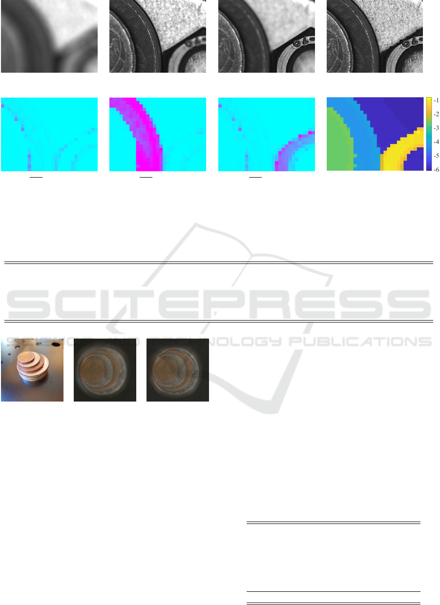
Figure 5: For the depth map generation, a focal stack of grayscale images at the same position but at different heights is used.

Three images for different heights are shown in a), b) and c). The corresponding focus measures are visualized in e), f) and g).

The ﬁnal depth map generated out of all 351 images for z = −17.5, −17.4, . . . , 17.5 mm is shown in h). Based on the depth

map a all-in-focus image (d) can be extracted out of the focal stack.

Table 2: Speciﬁcations of the acquired data and possible sample sizes.

grayscale camera UV-NIR spectrometer NIR spectrometer

Maximal sample size (x × y × z) 40 cm × 10 cm × 3 cm 40 cm × 8 cm × 3 cm 40 cm × 8 cm × 3 cm

Spatial resolution 3.57 µm 60 µm 60 µm

Spectral resolution - 0.254 nm 3.219 nm

Wavelengths used - 390 nm − 944 nm 944 nm − 1600 nm

Number of bands used 1 2196 206

(a) Nonplanar

sample: stack of

coins.

(b) Pseudo RGB

of ﬁxed height

hsi.

of adaptive height

hsi.

Figure 6: A hyperspectral image of the stack of coins shown

in (a) has been created in two different ways. First using a

ﬁxed heights as if the sample is planar. The second time

with a adaptive height based on a depth map created out of

grayscale images. Pseudo RGB images for both hyperspec-

tral images are shown in (b) and (c).

be downloaded at https://www.is.uni-due.de/datasets.

Both datasets consist of the three-dimensional array

of reﬂectance data, a list of classes, the pixel-wise

annotation (ground truth), and a pseudo RGB image

generated from the hyperspectral data. The datasets

have in common that the spectra show high intra-class

variability. This means that the classes cannot be dis-

tinguished by a naive approach like thresholding at

one wavelength.

4.1 Cereals Dataset

The cereals dataset shows an image of ﬁve differ-

ent types of cereal ﬂakes (oats, wheat, spelt, rice,

rye). The real world dimensions of the sample are

5 cm × 5 cm. The spatial resolution of the hypercube

is 500 × 500, the spectral domain consists of 2402

bands ranging from 380 nm to 1600 nm.

The whole hypercube is shown in ﬁgure 7a, the

pseudo RGB image in ﬁgure 7b and the annotation

is visualized in ﬁgure 7c. Three randomly selected

spectra of each class are plotted in ﬁgure 7d. Table 3

lists all classes and their number of occurrences.

Table 3: Classes of the cereals dataset.

label class number of samples

0 background 113,160

1 oat 22,380

2 rice 16,562

3 rye 28,481

4 spelt 33,613

5 wheat 35,804

total: 250,000

PHOTOPTICS 2022 - 10th International Conference on Photonics, Optics and Laser Technology

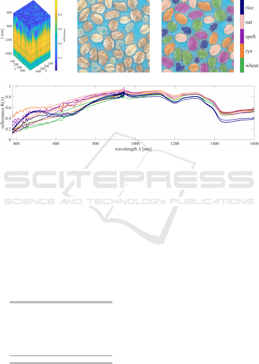
(a) Hypercube. (b) Pseudo RGB image. (c) Labels.

(d) Three (randomly selected) spectra from each class.

Figure 7: The cereals dataset presented in this paper contains ﬂakes made of oat, wheat, spelt, rice and rye. The sample has a

size of 5 cm× 5 cm, the hypercube (a) has the dimensions 500× 500 × 2402. Out of the hyperspectral data a pseudo RGB (b)

can be created. The annotation (c) is essential to train supervised classiﬁers on the dataset. Three (randomly selected) spectra

from each class are shown in (d). The colors of the spectra matches the labels (c).

4.2 Field Dataset

The ﬁeld dataset consists of materials occurring on

a ﬁeld (soil, two types of stones, leaf, ear, catkin,

branch). The sample dimensions are 2.66 cm ×

3.8 cm. The resolution of the hypercube (ﬁgure 8a)

is 266 × 380 × 2402.

The pseudo RGB image (ﬁgure 8b) and the anno-

tation of the dataset (ﬁgure 8c) are part of the dataset.

Three randomly selected spectra of each class are

plotted in ﬁgure 8d. Table 4 lists all classes and their

amount.

Table 4: Classes of the ﬁeld dataset.

label class number of samples

0 background 17,570

1 soil 41,136

2 stone 1 3,204

3 stone 2 7,987

4 ear 9,691

5 branch 5,175

6 catkin 2,111

7 leaf 14,206

total: 101,080

5 CONCLUSIONS

After summarizing the preliminary system for high-

resolution grayscale imaging and spectroscopy, we

presented the upgrades made to the system. Be-

sides new illuminations for both the gray value cam-

era and the spectrometers, these upgrades are mostly

software-based. We discussed the need and possi-

ble ways to do reﬂectance correction. The evaluation

suggested that a cubic model outperforms the ”sim-

ple100” approach, which is commonly used. There-

fore, a cubic approach should be preferred if enough

reﬂectance standards are available. Wavelength cor-

rection has been shown to be both essential and prac-

ticable using a polynomial regression approach.

We presented a procedure to acquire hyperspectral

images of non-planar samples with a spectrometer us-

ing a grayscale camera for focusing. The grayscale

camera has been used to provide a depth map of the

sample. The spectrometer objective is moved accord-

ingly to keep the sample in focus. This allows us to

acquire sharp hyperspectral images from non-planar

samples. Two datasets acquired like that are pub-

lished with this paper. The ﬁrst sample contains dif-

ferent sorts of cereal ﬂakes; the second sample con-

Combining a Grayscale Camera and Spectrometers for High Quality Close-range Hyperspectral Imaging of Non-planar Surfaces

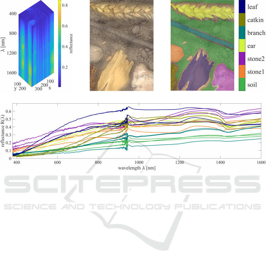
(a) Hypercube. (b) Pseudo RGB image. (c) Labels.

(d) Three (randomly selected) spectra from each class.

Figure 8: The ﬁeld dataset contains the classes soil, stones, leaf, ear, catkin and branch. The hypercube (a) has the dimensions

266 × 380 × 2402. Out of the hyperspectral data a pseudo RGB (b) can be created. The annotation (c) is used to train

supervised classiﬁers. Three (randomly selected) spectra from each class are shown in (d). The colors of the spectra matches

the labels (c).

sists of soil, stones, and plant materials occurring on

a ﬁeld. As we provide annotated datasets, they can be

used for supervised machine learning such as CNNs.

Possible future upgrades for the presented system

include a confocal illumination for the spectrometer

head. This would allow illuminating just the cur-

rently acquired part of the sample and therefore ex-

pand the range of possible samples to include light-

and heat-sensitive materials. Another improvement

could be made regarding the dichroic ﬁlter: An op-

tical path, which would introduce less noise at the

overlap between the spectrometers, would improve

the data quality even further. The impact of the ﬁl-

ter is currently the biggest drawback for the quality of

the data.

Besides these system-related considerations, our

future research will mainly deal with the analy-

sis of the acquired data. Here, our system offers

unique opportunities regarding the combination of

high-resolution grayscale images and hyperspectral

images with both a high spectral resolution and a

broad range of supported wavelengths.

REFERENCES

Baumgardner, M. F., Biehl, L. L., and Landgrebe, D. A.

(2015). 220 band aviris hyperspectral image data set:

June 12, 1992 indian pine test site 3.

Burger, J. and Geladi, P. (2005). Hyperspectral nir image

regression part i: calibration and correction. Journal

of Chemometrics.

Hagen, N. A. and Kudenov, M. W. (2013). Review of snap-

shot spectral imaging technologies. Optical Engineer-

ing.

Halicek, M., Dormer, J. D., Little, J. V., Chen, A. Y., and

Fei, B. (2020). Tumor detection of the thyroid and

salivary glands using hyperspectral imaging and deep

learning.

Hegemann, T., B

urger, F., and Pauli, J. (2017). Com-

bined high-resolution imaging and spectroscopy sys-

tem - a versatile and multi-modal metrology platform.

In Proceedings of the 5th International Conference on

Photonics, Optics and Laser Technology - Volume 1:

PHOTOPTICS,. SciTePress.

Herwig, J., Buck, C., Thurau, M., Pauli, J., and Luther, W.

(2012). Real-time characterization of non-metallic in-

clusions by optical scanning and milling of steel sam-

ples. In Optical Micro-and Nanometrology IV.

PHOTOPTICS 2022 - 10th International Conference on Photonics, Optics and Laser Technology

Kerekes, J. P. and Schott, J. R. (2007). Hyperspectral imag-

ing systems. Hyperspectral data exploitation: Theory

and applications.

Khan, H. A., Mihoubi, S., Mathon, B., Thomas, J.-B., and

Hardeberg, J. Y. (2018a). Hytexila: High resolution

visible and near infrared hyperspectral texture images.

Sensors.

Khan, M. J., Khan, H. S., Yousaf, A., Khurshid, K., and

Abbas, A. (2018b). Modern trends in hyperspectral

image analysis: A review. IEEE Access.

Klein, M. E., Aalderink, B. J., Padoan, R., Bruin, G. D., and

Steemers, T. A. G. (2008). Quantitative hyperspectral

reﬂectance imaging. Sensors.

Liang, H. (2012). Advances in multispectral and hyperspec-

tral imaging for archaeology and art conservation. Ap-

plied Physics A.

Liu, Y., Pu, H., and Sun, D.-W. (2017). Hyperspectral imag-

ing technique for evaluating food quality and safety

during various processes: A review of recent applica-

tions. Trends in food science & technology.

Lu, G. and Fei, B. (2014). Medical hyperspectral imaging:

a review. Journal of biomedical optics.

asi, R., Honkavaara, E., Lyytik

ainen-Saarenmaa, P.,

Blomqvist, M., Litkey, P., Hakala, T., Viljanen, N.,

Kantola, T., Tanhuanp

a, T., and Holopainen, M.

(2015). Using uav-based photogrammetry and hyper-

spectral imaging for mapping bark beetle damage at

tree-level. Remote Sensing.

Paoletti, M., Haut, J., Plaza, J., and Plaza, A. (2019). Deep

learning classiﬁers for hyperspectral imaging: A re-

view. ISPRS Journal of Photogrammetry and Remote

Sensing.

Park, B. and Lu, R. (2015). Hyperspectral imaging technol-

ogy in food and agriculture. Springer.

Pertuz, S., Puig, D., and Garcia, M. A. (2013). Analysis of

focus measure operators for shape-from-focus. Pat-

tern Recognition.

onen, I., Saari, H., Kaivosoja, J., Honkavaara, E., and

Pesonen, L. (2013). Hyperspectral imaging based

biomass and nitrogen content estimations from light-

weight uav. In Remote Sensing for Agriculture,

Ecosystems, and Hydrology XV. International Society

for Optics and Photonics.

Rasti, B., Hong, D., Hang, R., Ghamisi, P., Kang, X.,

Chanussot, J., and Benediktsson, J. A. (2020). Fea-

ture extraction for hyperspectral imagery: The evo-

lution from shallow to deep: Overview and toolbox.

IEEE Geoscience and Remote Sensing Magazine.

Yao, H. and Lewis, D. (2010). Spectral preprocessing and

calibration techniques. In Hyperspectral imaging for

food quality analysis and control. Elsevier.

Combining a Grayscale Camera and Spectrometers for High Quality Close-range Hyperspectral Imaging of Non-planar Surfaces