Neural Network Pruning based on Filter Importance Values
Approximated with Monte Carlo Gradient Estimation
Csan
´
ad S
´
andor
1,2 a
, Szabolcs P
´
avel
1,2 b
and Lehel Csat
´
o
1 c
1
Faculty of Mathematics and Informatics, Babes¸-Bolyai University, Kog
˘
alniceanu 1, Cluj-Napoca, Romania
2
Robert Bosch SRL, Somes¸ului 14, Cluj-Napoca, Romania
Keywords:
Neural Network Pruning, Filter Pruning, Structured Pruning, Neural Network Acceleration.
Abstract:
Neural network pruning is an effective way to reduce memory- and time requirements in most deep neu-
ral network architectures. Recently developed pruning techniques can remove individual neurons or entire
filters from convolutional neural networks, making these “slim” architectures more robust and more resource-
efficient. In this paper, we present a simple yet effective method that assigns probabilities to the network units
– to filters in convolutional layers and to neurons in fully connected layers – and prunes them based on these
values. The probabilities are learned by maximizing the expected value of a score function – calculated from
the accuracy – that ranks the network when different units are tuned off. Gradients of the probabilities are
estimated using Monte Carlo gradient estimation. We conduct experiments on the CIFAR-10 dataset with a
small VGG-like architecture as well as on the lightweight version of the ResNet architecture. The results show
that our pruning method has comparable results with different state-of-the-art algorithms in terms of parameter
and floating point operation reduction. In case of the ResNet-110 architecture, our pruning method removes
72.53% of the floating point operations and 68.89% of the parameters, that marginally surpasses the result of
existing pruning methods.
1 INTRODUCTION
Modern deep networks contain tens or hundreds of
layers and within each layer there are a plethora of pa-
rameters (He et al., 2016). While these large networks
can easily be used with sufficient memory and com-
puting power – generally via GPUs or TPUs –, their
use is complicated on resource-limited devices. The
commonly used – embedded or IoT – devices have
limited memory and computing power, they often run
on batteries, meaning that energy consumption is also
an important factor in the ergonomy of these devices.
To reduce the memory, energy and power consump-
tion of these networks, pruning can be applied on
them. Studies showed that more than half of the net-
work parameters can be removed such that their ac-
curacy is not affected (Han et al., 2016b; He et al.,
2019; Sandor et al., 2020).
Network pruning can be (1) unstructured pruning
and (2) structured pruning. In unstructured pruning
a
https://orcid.org/0000-0001-6666-0114
b
https://orcid.org/0000-0002-8825-2768
c
https://orcid.org/0000-0003-1052-1849
individual parameters – weights – are removed from
the network. This leads to highly compressed archi-
tectures with more than 90% of the parameters re-
moved (Han et al., 2016b), but the left-over param-
eters need to be stored in sparse matrices that require
special hardware (Han et al., 2016a) and special li-
braries (like sparse BLAS
1
) to be efficient. However,
these resources may not be always available. Struc-
tured pruning on the other hand focuses on remov-
ing groups of parameters (Li et al., 2016; He et al.,
2018, 2019): rows or columns from parameter matri-
ces (e.g. kernels), entire neurons or filters – we call
these functional units. Whilst there are less removed
parameters, the resulting architecture does not require
any special treatment.
This paper focuses on structured pruning of neural
networks: we approximate the importance of the net-
work functional units and remove the ones with small
scores. Our main contributions:
• We introduce binary random variables associated
with the functional units – we call them masks –,
1
cuSPARSE: the CUDA sparse matrix library, https://
docs.nvidia.com/cuda/cusparse
Sándor, C., Pável, S. and Csató, L.
Neural Network Pruning based on Filter Importance Values Approximated with Monte Carlo Gradient Estimation.
DOI: 10.5220/0010786700003124
In Proceedings of the 17th International Joint Conference on Computer Vision, Imaging and Computer Graphics Theory and Applications (VISIGRAPP 2022) - Volume 5: VISAPP, pages
315-322
ISBN: 978-989-758-555-5; ISSN: 2184-4321
Copyright
c
 2022 by SCITEPRESS – Science and Technology Publications, Lda. All rights reserved
315

parameterize and infer these hyper-parameters by
optimizing energy functions. We apply the log-
derivative trick and Monte Carlo gradient estima-
tion during the optimization.
• We show that the inferred values for the mask pa-
rameters can be used for pruning.
• We compare our method with different state-
of-the-art pruning algorithms and show that it
achieves comparable results with them.
2 PRUNING METHODS
Pruning is an active research field of neural network
compression (Blalock et al., 2020). The first pruning
techniques were presented in the beginning of 90s (Le
Cun et al., 1990; Hassibi et al., 1993). These meth-
ods used the Hessian of the loss function to remove
parameters. However, Hessian matrix calculation re-
quires huge computational power and a lot of mem-
ory. Due to these obstacles, it is hard to apply on
modern deep neural networks.
More recent work uses the magnitude of the
weights as a criterion (Han et al., 2015). After prun-
ing, the network is fine-tuned to regain the original
accuracy. The intuition is that small weights have
small impact, hence their absence will not affect over-
all performance. Han et al. (2016b) apply the un-
structured magnitude pruning and adds quantization
and Huffman coding to the pipeline. This way the
authors managed to reduce the VGG architecture of
Simonyan and Zisserman (2014) by a factor of 49.
Li et al. (2016) introduces a filter pruning ap-
proach with sensitivity analysis: filters in layers are
sorted and pruned based on their 
1
norms. This
process is stopped if the accuracy of the network
drops significantly. Yao et al. (2017) introduces a
compressor-critic framework, where the filter impor-
tance values are learned by a recurrent neural net-
work. This ”compressor” network takes the param-
eters of the original network and outputs probabilities
as importance values for the network units. To train
the compressor network, the expected value of the
original network’s loss is minimized over the proba-
bilities generated by the compressor. He et al. (2018)
presents a soft filter pruning approach where filters
with small 
2
norm are iteratively set to zero but they
are retrained afterwards – together with the other fil-
ters. This provides larger optimization space and the
pruning and retraining process has less dependence on
the pretrained model. While xprevious works utilize
the smaller norm less important criterion, He et al.
(2019) prunes deep neural networks based on filter
redundancy in layers: the geometric median of the
filters are calculated and the ones close to this me-
dian are removed from the network. Discrimination-
aware channel pruning (Liu et al., 2021) introduces
additional discrimination-aware losses to remove the
most discriminative channels. The paper introduces
the channel pruning as a sparsity-inducing optimiza-
tion problem and solve the convex objective with a
greedy algorithm.
Our method is similar to the work of Yao et al.
(2017) in that we use Monte Carlo method for the
gradient estimation, however we use a simple factor
model – using Bernoulli distributions – to approxi-
mate the probabilities – compared to their compres-
sor RNN network. This means our model is sim-
pler, more intuitive and requires less resources dur-
ing pruning. The way the pruning is defined could be
used as a dropout mechanism (Srivastava et al., 2014)
as well: while dropout uses predefined probabilities to
iteratively remove the units, our method learns these
values based on the importance of the units.
3 OUR PROPOSED METHOD
Consider a dataset D that contains N image and label
pairs (x
x
x
i
,y
i
)
N
i=1
. Let µ
W
(x
x
x) denote a neural network
that predicts y for the given x
x
x input, where W is the
set of network parameters.
2
We define network pruning as finding a binary
mask z
z
z ∈ {0, 1}
|W |
that sets part of the functional
units to 0, such that the accuracy remains sufficiently
high. This binary mask basically defines a subnet-
work in the original network. In pruning the question
is always how to find an optimal z
z
z mask?
To tackle this problem, we consider z
z
z a vector
of binary random variables where each z
i
indicates
whether the associated unit is active or not (i.e. is
dead). Let P
θ
θ
θ
(z
z
z) denote the joint probability distribu-
tion of the vector z
z
z, where θ
θ
θ are hyper-parameters and
let s(µ
W
(x
x
x|z
z
z)) be a score function of the mask z
z
z and
the input x
x
x. As defined above, x
x
x is an input image, but
it could be an image batch as well.
Our goal is to learn the P
θ
θ
θ
(z
z
z) probability distribu-
tion function such that the network score is as high
as possible. More formally, we want to maximize the
expected value of the score with respect to the proba-
bility distribution P
θ
θ
θ
(z
z
z):
2
Here W could “simply” be any vectorized form of the
parameters, but in the experiments we used e.g. filter ma-
trices as individual components and assigned a single mask
bit to this subset.
VISAPP 2022 - 17th International Conference on Computer Vision Theory and Applications
316

θ
θ
θ = argmax
θ
θ
θ
E
z
z
z∼P
θ
θ
θ
(z
z
z)
[s(µ
W
(x
x
x|z
z
z))] (1)
= argmax
θ
θ
θ
S(P
θ
θ
θ
),
where we defined the expected score as S(P
θ
θ
θ
).
To maximize the expected value, we need to op-
timize the parameterized probability distribution by
gradient ascent:
θ
θ
θ
k+1
= θ
θ
θ
k
+ α∇
θ
θ
θ
S(P
θ
θ
θ
)|
θ
θ
θ
k
(2)
However, calculating the expectation is not pos-
sible due to the large number of mask combinations
(in total 2
|W |
possibilities) where the network score
should be evaluated. Instead, we approximate the gra-
dient by developing Monte Carlo estimators (Robert
and Casella, 2010).
∇
θ
S(P
θ
θ
θ
) = ∇
θ
θ
θ
E
z
z
z∼P
θ
θ
θ
(z
z
z)
[s(µ
W
(x
x
x|z
z
z))]
=
Z
z
z
z
∇
θ
P
θ
θ
θ
(z
z
z)s(µ
W
(x
x
x|z
z
z))dz
z
z (3)
In Eq. (3) the gradient of the probability distribu-
tion appears (∇
θ
θ
θ
P
θ
θ
θ
(z
z
z)). This can be expressed using
the log-derivative trick:
∇
θ
θ
θ
P
θ
θ
θ
(z
z
z) = P
θ
θ
θ
(z
z
z)∇
θ
θ
θ
logP
θ
θ
θ
(z
z
z), (4)
and replacing Eq. (4) into Eq. (3), we get:
∇
θ
S(P
θ
θ
θ
) =
Z
z
z
z
P
θ
θ
θ
(z
z
z)∇
θ
θ
θ
logP
θ
θ
θ
(z
z
z)s(µ
W
(x
x
x|z
z
z))dz
z
z
=
E
z
z
z∼P
θ
θ
θ
(z
z
z)
[∇logP
θ
θ
θ
(z
z
z)s(µ
W
(x
x
x|z
z
z))], (5)
where we have the product of a probability distribu-
tion and a function that we can evaluate. Since in
Eq. (5) we have an expected value, we can rewrite
the expression and obtain that ∇
θ
θ
θ
S(P
θ
θ
θ
) is the expected
value of the score function times the gradient of the
log probability distribution.
Using the Monte Carlo method, we can approxi-
mate the gradient by deriving a general-purpose esti-
mator using N samples from the P
θ
θ
θ
(z
z
z) distribution:
∇
θ
θ
θ
S(P
θ
θ
θ
) ≈
1
N
N
∑
i=1
∇
θ
logP
θ
θ
θ
(z
z
z
i
)s(µ
W
(x
x
x|z
z
z
i
)) (6)
Since the estimated gradient can have higher vari-
ance, the convergence of the optimization can be
slower. To tackle this, we apply simple variance re-
duction techniques following the work of Yao et al.
(2017): we subtract the moving average of the score
from the actual score value and divide it by
√
1 −v,
where v denotes the variance of the score. We used the
above formulation in our algorithm (see Section 3.3).
3.1 Score of the Network
Eq. (1) contains a function that scores the network
when a z
z
z
i
mask is applied on it. This score has to be
high when the network performs ”well” and low oth-
erwise. To calculate the score for a given z
z
z
i
mask, the
network is evaluated on a random image batch from
the validation set (meaning that we train the proba-
bility distribution on the validation set). We exper-
iment with 3 different score functions and measure
how quickly the probabilities converge to 0 or 1 and
how the pruning affects the network accuracy.
The loss-score function is used from the work
of Sandor et al. (2020):
s
i
=
L
max
−L
i
L
max
−L
min
, (7)
where L
i
is the network loss with the z
z
z
i
mask, L
min
and L
max
are the minimum and maximum values
among the L
i
losses. This way the score is 1 when the
network loss is the smallest (network performs well)
and 0 when the loss is the highest.
The acc-score uses the accuracy as a score func-
tion. Let X denote a random batch of images from the
validation set and Acc(µ
W
(X |z
z
z
i
)) denote the network
accuracy on the image batch when z
z
z
i
mask is applied
on it. Then the score of the z
z
z
i
mask is simply:
s
i
= Acc(µ
W
(X |z
z
z
i
)) (8)
The exp-acc-score applies a scaling and an expo-
nential function on the accuracy:
s
i
= exp(
Acc(µ
W
(X |z
z
z
i
))
β
) (9)
While the accuracy can be used as a score func-
tion, it cannot capture fine-grained details: if z
z
z
i
and
z
z
z
j
differs only in a single value, the scores could be
very close to each other. This results small difference
between the gradients as well, resulting slow conver-
gence during the factor model optimization. The exp-
acc-score function increases the distance between the
scores when the accuracy values are similar.
The experiments with the different score functions
are presented in section 4.1.
3.2 Probability Distribution
An important question is how to represent the proba-
bility distribution over the set of random variables z?
For simplicity, we assume independence between the
elements and define the probability distribution as a
product of Bernoulli distributions:
P
θ
θ
θ
(z
z
z) =
∏
i
p
z
i
i
(1 − p
i
)
1−z
i
, (10)
Neural Network Pruning based on Filter Importance Values Approximated with Monte Carlo Gradient Estimation
317

where the probability that z
i
= 1 depends on the θ
i
parameter: P
θ
i
(z
i
= 1) = p
i
= σ(θ
i
).
Using the factor model from Eq. (10), the log
probability in Eq. (6) can be written as:
logP
θ
θ
θ
(z
z
z) = log
∏
i
p
z
i
i
(1 − p
i
)
1−z
i
(11)
=
∑
i
z
i
log p
i
+ (1 −z
i
)log(1 −p
i
)
3.3 Network Pruning Algorithm
To use the factor model as a probability distribution,
we assume independence between the network units
(neurons and filters). Since this assumption is clearly
not true in case of a multilayer network, we assume
independence only between units from the same layer.
This way, we prune the network layer by layer, learn-
ing separate probability distributions for each layer. A
formalized version is presented in Algorithm 1.
Algorithm 1: Network pruning.
Require: µ
W
pre-trained network
1: l ← index of first or last layer
2: while stopping condition not met do
3: initialize P
θ
θ
θ
(z
z
z) for layer l
4: for some predefined steps do
5: sample {z
z
z
1
,...,z
z
z
N
} masks from P
θ
θ
θ
(z
z
z)
6: calculate ∇
θ
θ
θ
S(P
θ
θ
θ
)  from Eq. (6)
7: update θ
θ
θ  from Eq. (2)
8: prune layer l based on P
θ
θ
θ
(z
z
z)
9: fine-tune µ
W
10: l ← next layer index
4 EXPERIMENTS
We analyze our pruning algorithm on different archi-
tectures trained on the CIFAR-10 (Krizhevsky et al.,
2009) dataset.
Similar to (Frankle and Carbin, 2019), we use a
small VGG-like (Simonyan and Zisserman, 2014) ar-
chitecture with two convolutional layers, a max pool
layer and three fully connected layers. Both con-
volutional layers contain 64, 3 ×3 filters while the
fully connected layers have 256, 256 and 10 neu-
rons respectively. In the hidden layers ReLU ac-
tivation function is used. The network is trained
on the CIFAR-10 dataset for 10 epochs (using
Adam optimizer (Kingma and Ba, 2015) with 2 ×
10
−4
learning rate and early stopping condition) and
reaches 69.76% accuracy on the validation dataset
and 68.95% on the test dataset.
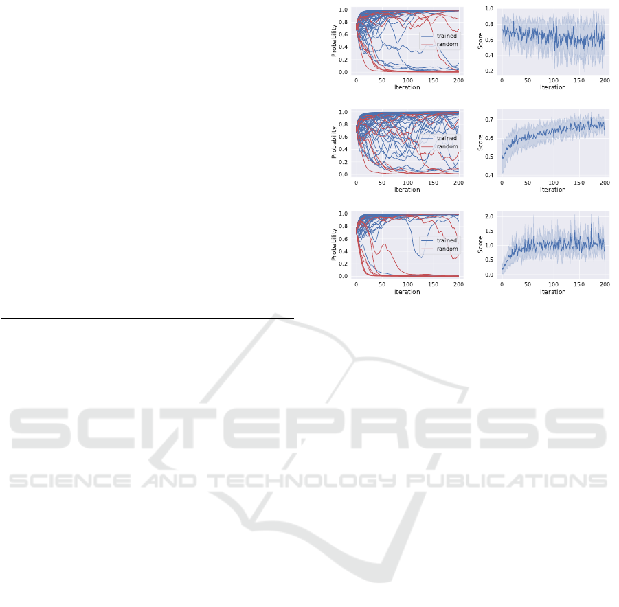
Figure 1: Left: Inferred probabilities for the 74 filters in the
first convolutional layer (10 of them are filters with random
weights). Right: standard deviation of the scores during
the training process. Top: loss-score function, middle: acc-
score function, bottom: exp-acc-score function.
4.1 Score Function
To analyze the different score functions presented in
section 3.1, we prune the trained VGG-like network:
First, we insert 10 extra filters (containing random
weights) in the first convolutional layer. Then we
prune the network and measure the true positive rate:
how many extra filters are pruned from the network.
A score function is better if the pruning algorithm can
identify more filters with random weights.
In case of each function, we train our factor model
from Eq. (10) for 200 iterations and remove the filters
with small probabilities (we use 0.2 as a threshold).
We repeat the process until at least 10 filters are re-
moved from the network and measure the validation
and test accuracy of the pruned networks. For each
of the 3 score functions we repeat the experiment 5
times and report the average validation and test accu-
racy, the number of removed filters and the true posi-
tives (number of removed filters that contain random
weights). Results are reported in Table 1. As the table
shows, the pruning method detects part of the inserted
random filters. However, the true positive rate and the
pruned network accuracy varies. When the network
loss and accuracy is used to calculate the score (first
2 rows in the table), on average more then 11 filters
are removed from the network. However, around 6-7
of them are true positives, that means 30 −40% of the
removed units contains trained weights. In these cases
the network accuracy decreases quite heavily as well:
VISAPP 2022 - 17th International Conference on Computer Vision Theory and Applications
318

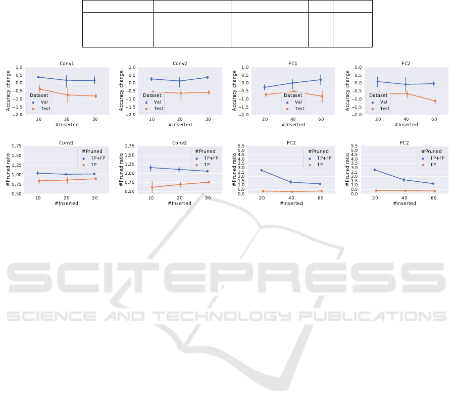
Table 1: Pruning results using the three different score functions. The validation and test accuracy, true and false positives
(Tp and Fp) are averages from 5 different experiments. We insert 10 random filters in each experiment, thus the ideal case
would be that the algorithm prunes only those 10 filters.
Score function Val. acc. (%) Test acc. (%) Tp Tp+Fp
loss-score 68.84 (↓ 0.91%) 67.76 (↓ 1.18%) 6.8 11.2
acc-score 67.99 (↓ 1.76%) 66.72 (↓ 2.22%) 6.0 11.0
exp-acc-score 70.11 (↑ 0.35%) 68.56 (↓ 0.38%) 8.4 10.2
Figure 2: Up: Accuracy change of the pruned networks when different number of filters (10, 20, 30) or neurons (20, 40, 60)
are inserted into the layers. Down: true and false positive rates of the pruning.
0.91% and 1.76% on the validation set and 1.18% and
2.22% on the test set. Results are more promising in
case of the exponential score function: on average 8.4
from 10 random filters are found by the algorithm and
the pruned network accuracy increases by 0.35% on
the validation set and decreases only 0.38% on the test
dataset.
In Figure 1, we present the dynamics of the in-
ferred probabilities and scores during the factor model
training. The left figures show how the mask proba-
bilities converge to 0 and 1 during this process. It is
easy to see that the convergence is much faster in case
of the loss-score and exp-acc-score functions (top and
bottom). Using these functions, the values quickly
moves close to 0 or 1 depending on the filter’s impor-
tance. Slow convergence with the acc-score function
is related to the value of the scores (right figure): dur-
ing the factor model training the standard deviation
of the scores decreases. This means that the differ-
ence between the gradients decreases as well, leading
to slow convergence. The standard deviation of the
scores is much higher in case of the loss-score and
exp-acc-score functions. This is important, since as
the probabilities start to converge (the network ac-
curacy approximate the original accuracy), a small
change on the z
z
z
i
mask leads to higher change on the
score – meaning the difference between the gradients
are higher.
While the dynamics of the probabilities with loss-
score and exp-acc-score functions are similar (top and
bottom figures), the values converges a bit quicker
with the latter. Moreover, as Table 1 shows, the re-
sult are also better with this function. This is be-
cause exp-acc-score function provides consistent val-
ues during the training process while the values of
loss-score depends on L
min
and L
max
: the same z
z
z
i
mask can have different scores in different training
iterations as L
min
and L
max
changes - which is very
likely, since the masks are randomly sampled. This
varying score affects the gradients that leads to slower
convergence.
4.2 Pruning Randomly Inserted Filters
from Trained Networks
Based on the presented experiments in section 4.1,
we select the exp-acc-score function and examine the
pruning algorithm on different layers of the VGG-like
network. Similar to section 4.1, we insert randomly
initialized filters and neurons into the trained VGG-
like network, however, we vary the number of ran-
dom filters and the target layers as well. In case of
the convolutional layers, we insert 10, 20 and 30 ran-
dom filters while in the fully connected layers we in-
sert 20, 40 and 60 random neurons one after another.
We repeat each experiment 5 times and report the av-
erage change of the validation and test accuracy (be-
tween the pruned and original networks), the average
number of removed filters (TP + FP) and the average
number of the removed random filters (TP). Figure 2
Neural Network Pruning based on Filter Importance Values Approximated with Monte Carlo Gradient Estimation
319

presents the results of this experiment.
The first 4 figures show the accuracy change of
the pruned networks compared to the original net-
work accuracy (trained network, no random filters in-
serted). Since the probability distribution is optimized
to maximize the expected value of the scores calcu-
lated on the validation set, the validation accuracy of
the pruned network outperforms the validation accu-
racy of the original network in almost all 4 cases. This
validates that Eq. (6) correctly estimates the gradi-
ent and the gradient method can increase the expected
value of the score. In case of the test accuracy, a drop
between 0.5% and 1.2% can be detected, and the gap
is slowly increases with the number of inserted filters.
This means the overfitting becomes stronger as more
random filters are inserted into the network.
Figures from the bottom show the number of re-
moved filters (TP+FP) and number of removed ran-
dom filters (TP) among the 4 experiments. The first
observation here is that filters in the first layer are
more important than filters in the second layer: while
the true positive rate is around 80% in the first layer, it
is between 60 −75% at the second layer. This means
that more trained filters are removed from the second
layer, but the accuracy values remain similar (or even
better in case of the second layer). At the fully con-
nected layers the true positive rate decreases below
50%. These layers contain more than 256 neurons
but only a fraction of them contributes to the correct
output. The pruning algorithm can ”pick” almost ran-
domly from the pool and the accuracy still remains
near to the original accuracy.
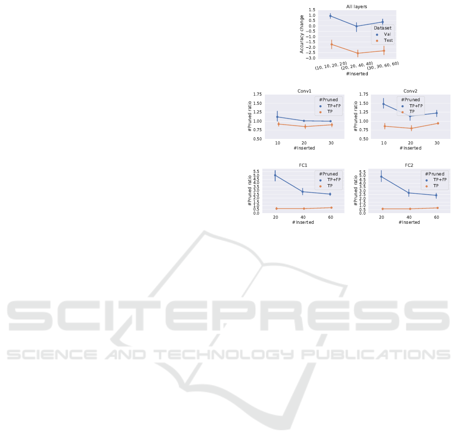
In our second experiment we use the same net-
work but instead of targeting only a single layer we
insert randomly initialized filters into all the network
layers. This problem is more challenging since filters
have influence to each other through the layers. As
presented in section 3.3, we apply sequential prun-
ing: the algorithm prunes the layers one by one and
repeats the process until the target size is not reached
(Figure 3).
The results show that the algorithm can find more
than 75% of the random filters in the convolutional
layers and more than 50% of the neuron in the fully
connected layers. While these values are similar with
the results of the previous experiment, here the test
accuracy drop increases to 1.5 −3% (Figure 3, top).
4.3 Pruning the ResNet Architecture
Next, we are testing the ResNet (He et al., 2016) net-
work. This is an efficient CNN architecture that ap-
plies residual blocks and “shortcut connections” for
better propagation of the error signal. The residual
Figure 3: Up: Accuracy change of the pruned networks
when different number of units are inserted into the four
layers. Middle and down: true and false positive rates of
the pruning at different layers.
block contains two sets of convolutional, batch nor-
malization and ReLU layers, such that the output of a
layer is fed into the input of the next layer. To prune
the units in this residual block, we insert mask layers
following the work of Sandor et al. (2020): the first
mask layer is inserted after the first ReLU layer while
the second mask layer is inserted before the shortcut
connection.
Training Details: We experiment with the ResNet-
32, 56 and 110 architectures. We train the networks
following the work of He et al. (2016), with the fol-
lowing modifications: we change the initial 0.1 learn-
ing rate to 0.01 and 0.001 at epochs 100, and 150 and
stop the training at 200 epochs. During training we
apply cropping and horizontal flip as data augmenta-
tion. The network is trained on a 45K train set, a 5K
validation set is used for training the parameterized
probability distribution.
Pruning Details: Pruning is applied based on the al-
gorithm presented in section 3.3. We start the process
from the network’s first layer and calculate the prob-
abilities layer by layer. In each layer, we train the
probability distribution (Eq. 10) in 200 iteration such
that in each iteration 50 masks are sampled and their
corresponding scores are calculated. In each iteration
the gradients are estimated – using Eq. (6) – and the
parameters are updated – using Eq. (2). After 200 it-
erations units with small probability are turned off –
here we follow the work of Sandor et al. (2020): we
drop the least important units such that the accuracy
VISAPP 2022 - 17th International Conference on Computer Vision Theory and Applications
320

Table 2: Comparison of pruned ResNet with the results from the literature.
ResNet Method
Accuracy (%) ↓(%)
Baseline Pruned Diff. ↓ FLOPs Params.
32
SFP (He et al., 2018) 92.63 92.08 0.55 41.5 41.24*
FPGM (He et al., 2019) 92.63 92.82 -0.19 53.2 53.2*
LFE (Sandor et al., 2020) 92.97 92.42 0.55 46.4 49.35
Ours 92.97 92.29 0.68 50.22 43.65
56
(Li et al., 2016) 93.04 93.06 -0.02 27.6 13.7
SFP (He et al., 2018) 93.59 93.35 0.1 47.14 52.6*
ThiNet (Luo et al., 2019) 93.8 92.98 0.82 49.78 49.67
FPGM (He et al., 2019) 93.59 93.49 0.1 47.14 52.6*
LFE (Sandor et al., 2020) 93.44 93.18 0.26 57.64 68.14
Adapt-DCP (Liu et al., 2021) 93.74 93.77 -0.03 68.48 54.80
Ours 93.44 93.08 0.36 64.22 57.79
110
(Li et al., 2016) 93.53 93.3 0.23 38.6 32.40
SFP (He et al., 2018) 93.68 93.86 -0.18 40.8 40.72*
FPGM (He et al., 2019) 93.68 93.85 -0.17 52.3 52.7*
LFE (Sandor et al., 2020) 94.05 93.48 0.57 63.68 60.08
Ours 94.05 93.45 0.6 72.53 68.89
*Parameter drop percentage is not reported in the paper. These values are calculated from other
available information (e.g. ”40% of the filters are selected”).
drop on the validation dataset is less than 1.0%. After
a layer is pruned, we apply fine-tuning for 10 epochs.
Finally, when no more filters can be removed,
we retrain the network for 100 epochs by setting the
learning rate to 0.1 and decrease to 0.01 and 0.001 at
epochs 40 and 60.
Results: We report the pruning results of the
ResNet architecture in Table 2. The algorithm re-
moves 43.65% of the parameters and 50.22% of the
floating point operations (FLOPs) from the ResNet-
32 architecture. While these values outperform the
results of He et al. (2018) in terms of parameter and
FLOPs reduction, remains below the results of He
et al. (2019) and Sandor et al. (2020). While the prun-
ing results are modest with the smaller ResNet, they
are more promising with the ResNet-56 and ResNet-
110 versions. We manage to remove 64.22% of
the FLOPS and 57.79% of the parameters from the
ResNet-56 with only 0.36 accuracy drop. These val-
ues outperform most of the results reported by the pa-
pers selected for comparison: only the FLOPs reduc-
tion result of Liu et al. (2021) and the parameter re-
duction result of Sandor et al. (2020) can outperform
our algorithm. In case of the ResNet-110 architecture,
our pruning algorithm removes more than two thirds
of the floating point operations (72.53%) and the pa-
rameters (68.89%). These values surpass the results
of the other papers with a significant margin.
5 CONCLUSIONS
In this paper, we described a structured pruning al-
gorithm that approximates the importance probability
of network units using Monte Carlo gradient estima-
tion. To calculate the importance values, we intro-
duced a function that scores the performance of dif-
ferent subnetworks. A subnetwork is defined as a bi-
nary masks that specifies the active and inactive units
in the network. Given a set of score and their cor-
responding subnetwork – binary mask –, we maxi-
mize the expected score of the network by optimizing
the probability distribution of the masks using esti-
mated gradients from the Monte Carlo method. Based
on the importance values, our method applies prun-
ing on the network and produces a compressed model
with parameters stored in smaller, dense matrices. We
showed the effectiveness of our pruning algorithm on
the CIFAR-10 dataset with a small VGG-like archi-
tecture as well as on different versions of the ResNet
architecture. The experiments show that our algo-
rithm has comparable results with current state-of-
the-art pruning methods.
REFERENCES
Blalock, D. W., Ortiz, J. G., Frankle, J., and Guttag, J.
(2020). What is the state of neural network pruning?
ArXiv, abs/2003.03033.
Frankle, J. and Carbin, M. (2019). The lottery ticket hy-
pothesis: Finding sparse, trainable neural networks.
In ICLR’2019.
Neural Network Pruning based on Filter Importance Values Approximated with Monte Carlo Gradient Estimation
321

Han, S., Liu, X., Mao, H., Pu, J., Pedram, A., Horowitz, M.,
and Dally, W. (2016a). Eie: Efficient inference en-
gine on compressed deep neural network. ISCA’2016,
pages 243–254.
Han, S., Mao, H., and Dally, W. J. (2016b). Deep compres-
sion: Compressing deep neural network with prun-
ing, trained quantization and huffman coding. In
ICLR’2016.
Han, S., Pool, J., Tran, J., and Dally, W. J. (2015). Learn-
ing both weights and connections for efficient neural
networks. In NIPS’2015, NIPS’15, pages 1135–1143,
Cambridge, MA, USA.
Hassibi, B., Stork, D. G., Wolff, G., and Watanabe, T.
(1993). Optimal brain surgeon: Extensions and
performance comparisons. In NIPS’1993, NIPS’93,
pages 263–270.
He, K., Zhang, X., Ren, S., and Sun, J. (2016). Deep resid-
ual learning for image recognition. In CVPR’2016,
pages 770–778.
He, Y., Kang, G., Dong, X., Fu, Y., and Yang, Y. (2018).
Soft filter pruning for accelerating deep convolutional
neural networks. In IJCAI’2018, pages 2234–2240.
He, Y., Liu, P., Wang, Z., Hu, Z., and Yang, Y. (2019). Filter
pruning via geometric median for deep convolutional
neural networks acceleration. In CVPR’2019.
Kingma, D. P. and Ba, J. (2015). Adam: A method for
stochastic optimization. In ICLR’2015.
Krizhevsky, A., Nair, V., and Hinton, G. (2009). Learning
multiple layers of features from tiny images. Techni-
cal report, Faculty of Computer Science, University of
Toronto.
Le Cun, Y., Denker, J. S., and Solla, S. A. (1990). Optimal
brain damage. In NIPS’1990, pages 598–605.
Li, H., Kadav, A., Durdanovic, I., Samet, H., and Graf, H. P.
(2016). Pruning filters for efficient convnets. CoRR,
abs/1608.08710.
Liu, J., Zhuang, B., Zhuang, Z., Guo, Y., Huang, J., Zhu,
J., and Tan, M. (2021). Discrimination-aware network
pruning for deep model compression. TPAMI’2021,
PP:(early access).
Luo, J.-H., Zhang, H., Zhou, H.-Y., Xie, C.-W., Wu, J., and
Lin, W. (2019). Thinet: Pruning cnn filters for a thin-
ner net. TPAMI’2019, 41(10):2525–2538.
Robert, C. P. and Casella, G. (2010). Monte Carlo Statisti-
cal Methods.
Sandor, C., Pavel, S., and Csato, L. (2020). Pruning CNN’s
with Linear Filter Ensembles. In ECAI’2020, volume
325 of Frontiers in Artificial Intelligence and Applica-
tions, pages 1435–1442.
Simonyan, K. and Zisserman, A. (2014). Very deep con-
volutional networks for large-scale image recognition.
CoRR, abs/1409.1556.
Srivastava, N., Hinton, G., Krizhevsky, A., Sutskever, I.,
and Salakhutdinov, R. (2014). Dropout: A sim-
ple way to prevent neural networks from overfitting.
JMLR’2014, 15(56):1929–1958.
Yao, S., Zhao, Y., Zhang, A., Su, L., and Abdelzaher, T.
(2017). Deepiot: Compressing deep neural network
structures for sensing systems with a compressor-
critic framework. In SenSys’2017.
VISAPP 2022 - 17th International Conference on Computer Vision Theory and Applications
322