Safe Policy Improvement Approaches

on Discrete Markov Decision Processes

Philipp Scholl

1,2

, Felix Dietrich

, Clemens Otte

and Steffen Udluft

Department of Mathematics, Ludwig-Maximilian-University of Munich, Munich, Germany

Learning Systems, Siemens Technology, Munich, Germany

Department of Informatics, Technical University of Munich, Munich, Germany

Keywords:

Risk-sensitive Reinforcement Learning, Safe Policy Improvement, Markov Decision Processes.

Abstract:

Safe Policy Improvement (SPI) aims at provable guarantees that a learned policy is at least approximately as

good as a given baseline policy. Building on SPI with Soft Baseline Bootstrapping (Soft-SPIBB) by Nadjahi et

al., we identify theoretical issues in their approach, provide a corrected theory, and derive a new algorithm that

is provably safe on ﬁnite Markov Decision Processes (MDP). Additionally, we provide a heuristic algorithm

that exhibits the best performance among many state of the art SPI algorithms on two different benchmarks.

Furthermore, we introduce a taxonomy of SPI algorithms and empirically show an interesting property of two

classes of SPI algorithms: while the mean performance of algorithms that incorporate the uncertainty as a

penalty on the action-value is higher, actively restricting the set of policies more consistently produces good

policies and is, thus, safer.

1 INTRODUCTION

Reinforcement learning (RL) in industrial control ap-

plications such as gas turbine control (Schaefer et al.,

2007) often requires learning a control policy solely

on pre-recorded observation data, known as batch or

ofﬂine RL (Lange et al., 2012; Fujimoto et al., 2019;

Levine et al., 2020). This is necessary because an on-

line exploration on the real system or its simulation is

not possible. Assessing the true quality of the learned

policy is difﬁcult in this setting (Hans et al., 2011;

Wang et al., 2021). Thus, Safe Policy Improvement

(Thomas, 2015; Nadjahi et al., 2019) is an attractive

resort as it aims at ensuring that the learned policy is,

with a high probability, at least approximately as good

as a baseline policy given by, e.g., a conventional con-

troller.

Safety is an overloaded term in Reinforcement

Learning as it can refer to the inherent uncertainty,

safe exploration techniques or parameter uncertainty

(Garc

ıa and Fernandez, 2015). In this paper we focus

on the latter.

1.1 Related Work

Many of the existing Safe Policy Improvement (SPI)

algorithms utilize the uncertainty of state-action pairs

in one of the two following ways (see also Figure 1):

1. The uncertainty is applied to the action-value

function to decrease the value of uncertain ac-

tions.

2. The uncertainty is used to restrict the set of poli-

cies that can be learned.

Thomas (2015) introduced High Conﬁdence Pol-

icy Improvement (HCPI), an algorithm utilizing con-

centration inequalities on the importance sampling es-

timate of the performance of learned policies to en-

sure that the new policy is better than the baseline

with a high probability. As HCPI simply rejects poli-

cies where the conﬁdence intervals give no certain

improvement, they essentially restrict the set of pos-

sible policies. This restriction is clearer for Robust

MDP (Nilim and El Ghaoui, 2003), which computes

the policy with the best worst-case performance for

all transition probabilities in a convex set, which is

chosen such that the true transition probabilities are

part of it with a high probability.

Petrik et al. (2016) showed that maximizing the

difference between the new policy and a baseline

policy on a rectangular uncertainty set of the tran-

sition probabilities is NP-hard and, thus, derived

the approximation Reward-adjusted MDP (RaMDP).

RaMDP applies the uncertainty to penalize the reward

142

Scholl, P., Dietrich, F., Otte, C. and Udluft, S.

Safe Policy Improvement Approaches on Discrete Markov Decision Processes.

DOI: 10.5220/0010786600003116

In Proceedings of the 14th International Conference on Agents and Artiﬁcial Intelligence (ICAART 2022) - Volume 2, pages 142-151

ISBN: 978-989-758-547-0; ISSN: 2184-433X

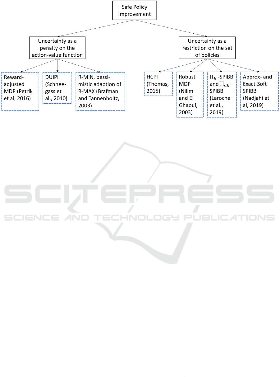
Figure 1: Taxonomy of SPI algorithms.

and, therefore, the action-value function. Laroche

et al. (2019) extended this algorithm by a hyper-

parameter which controls the inﬂuence of the uncer-

tainty. RaMDP computes the uncertainty simply as

a function of the number of visits to a state-action

pair. A more sophisticated approach to estimate the

uncertainty is taken for Diagonal Approximation of

Uncertainty Incorporating Policy Iteration (DUIPI) in

Schneegass et al. (2010), which estimates the standard

deviation of the action-value function and applies this

as a penalty to the action-value function. Utilizing the

uncertainty as an incentive instead of a penalty results

in an explorative algorithm. Applying this correspon-

dence between exploratory and safe behavior to fur-

ther algorithms, one can easily adapt the efﬁciently

exploring R-MAX (Brafman and Tennenholtz, 2003),

which assigns the highest value possible to all rarely

visited state-action pairs, to its risk averse counterpart

that we denote as R-MIN. This algorithm simply sets

the action-value to the lowest possible value instead

of the highest one for rarely visited state-action pairs.

Returning back to algorithms restricting the policy

set, Laroche et al. (2019) only allow deviations from

the baseline policy at a state-action pair if the uncer-

tainty is low, otherwise it remains the same. They

propose two algorithms: Π

-SPIBB, which is prov-

ably safe, and Π

≤b

-SPIBB, which is a heuristic re-

laxation. Both are tested against HCPI, Robust MDP,

and RaMDP. HCPI and Robust MDP are strongly out-

performed by the others and, while the mean perfor-

mance of RaMDP is very good, its safety is inferior

to both SPIBB algorithms. Nadjahi et al. (2019) con-

tinue this line of work and relax the hard bootstrap-

ping to a softer version, where the baseline policy can

be changed at any state-action pair, but the amount

of possible change is limited by the uncertainty at

this state-action pair. They claim that these new al-

gorithms, called Safe Policy Improvement with Soft

Baseline Bootstrapping (Soft-SPIBB), are also prov-

ably safe, a claim that is repeated in Sim

ao et al.

(2020) and Leurent (2020). Furthermore, they extend

the experiments from Laroche et al. (2019) to include

the Soft-SPIBB algorithms, where the empirical ad-

vantage of these algorithms becomes clear.

1.2 Our Contributions

We investigate the class of Soft-SPIBB algorithms

(Nadjahi et al., 2019) and show that they are not

provably safe. Hence, we derive the adaptation Adv-

Approx-Soft-SPIBB which is provably safe. We also

develop the heuristic Lower-Approx-Soft-SPIBB, fol-

lowing an idea presented in Laroche et al. (2019). Ad-

ditionally, we conduct experiments to test these new

versions against their predecessors and add further

uncertainty incorporating algorithms (Brafman and

Tennenholtz, 2003; Schneegass et al., 2010) which

were not considered in Laroche et al. (2019) and Nad-

jahi et al. (2019). Here, we also show how the taxon-

omy illustrated in Figure 1 proves to be helpful, as

both classes of algorithms present different behavior.

The code for the algorithms and experiments can be

found in the accompanying repository.

1.3 Outline

The next section introduces the mathematical frame-

work necessary for the later sections. Section 3 begins

with the work done by Nadjahi et al. (2019) and ends

https://github.com/Philipp238/Safe-Policy-Improvem

ent-Approaches-on-Discrete-Markov-Decision-Processes

Safe Policy Improvement Approaches on Discrete Markov Decision Processes

143

with a discussion and proof of the shortcomings of the

given safety guarantees. In Section 4 we deduce the

new algorithms, which will be tested against various

competitors on two benchmarks in Section 5.

2 MATHEMATICAL

FRAMEWORK

The control problem we want to tackle with reinforce-

ment learning consists of an agent and an environ-

ment, modeled as a ﬁnite Markov Decision Process

(MDP). A ﬁnite MDP M

∗

is represented by the tu-

ple M

∗

= (S , A,P

∗

, R

∗

, γ), where S is the ﬁnite state

space, A the ﬁnite action space, P

∗

the unknown tran-

sition probabilities, R

∗

the unknown stochastic reward

function, the absolute value of which is assumed to be

bounded by R

max

, and 0 ≤γ < 1 is the discount factor.

The agent chooses action a ∈ A with probability

π(a|s) in state s ∈S , where π is the policy controlling

the agent. The return at time t is deﬁned as the dis-

counted sum of rewards G

∑

i=t

i−t

∗

, a

), with

T the time of termination of the MDP. As the reward

function is bounded the return is bounded as well,

since |G

| ≤

max

1−γ

. So, let G

max

be a bound on the ab-

solute value of the return. The goal is to ﬁnd a policy

π which optimizes the expected return, i.e., the state-

value function V

∗

(s) = E

= s] for the initial

state s ∈ S . Similarly, the action-value function is de-

ﬁned as Q

∗

(s, a) = E

= s, A

= a].

Given data D = (s

, a

, r

, s

′

)

j=1,...,n

collected by

the baseline policy π

, let N

(s, a) denote the num-

ber of visits of the state-action pair (s, a) in D and

M = (S , A ,

R, γ) the Maximum Likelihood Estima-

tor (MLE) of M

∗

where

P(s

′

|s, a) =

∑

=s,a

=a,r

′

)∈D

(s, a)

(1)

and

R(s, a) =

∑

=s,a

=a,r

′

)∈D

(s, a)

. (2)

3 THE SOFT-SPIBB PARADIGM

The idea in Nadjahi et al. (2019) is to estimate the

uncertainty in the state-action pairs and bound the

change in the baseline policy accordingly.

3.1 Preliminaries

To bound the performance of the new policy it is nec-

essary to bound the estimate of the action-value func-

tion. In Nadjahi et al. (2019) this is done for Q

by applying Hoeffding’s inequality. However, Ho-

effding’s inequality is only applicable for the arith-

metic mean of independent, bounded random vari-

ables, thus, we deﬁne

(s, a) =

∑

i=1

as the

Monte Carlo estimate of the action-value function,

where t

, ...,t

are times such that (S

, A

) = (s, a) for

all i = 1, ..., n. See Scholl (2021) for a discussion of

the (approximate) independence of G

. Following the

proof in Appendix A.2 in Nadjahi et al. (2019) yields

that

∗

(s, a) −

(s, a)| ≤ e

(s, a)G

max

(3)

holds with probability 1 −δ for all state-action pairs.

Here, e

is the error function computing the uncer-

tainty of one state-action pair and is given by

(s, a) =

(s, a)

log

2|S ||A|

. (4)

Analogously,

||P(·|s, a) −

P(·|s, a)||

≤ e

(s, a), (5)

holds with probability 1 −δ where

(s, a) =

(s, a)

log

2|S ||A|2

|A|

. (6)

The error functions are used to quantify the uncer-

tainty of each state-action pair.

Deﬁnition 1. A policy π is (π

, ε, e)-constrained w.r.t.

a baseline policy π

, an error function e and a hyper-

parameter ε > 0, if

∑

a∈A

e(s, a)|π(a|s) −π

(a|s)| ≤ ε (7)

holds for all states s ∈ S .

So, if a policy π is (π

, ε, e)-constrained, it means

that the l

-distance between π and π

′

, weighted by

some error function e, is at most ε. To utilize Equation

3 later the following property is also necessary:

Deﬁnition 2. A policy π is π

-advantageous w.r.t. the

function Q : S ×A → R, if

∑

Q(s, a)π(a|s) ≥

∑

Q(s, a)π

(a|s) (8)

holds for all states s ∈ S .

Note that this is an extension of Deﬁnition 3 in

Nadjahi et al. (2019) to arbitrary functions and can,

thus, be used for

. Interpreting Q as some kind

of action-value function, Deﬁnition 2 gives that the

policy π chooses higher valued actions than policy π

′

for every state.

ICAART 2022 - 14th International Conference on Agents and Artiﬁcial Intelligence

144

3.2 The Algorithms

The new class of algorithms (Nadjahi et al., 2019) in-

troduce make use of the classical Policy Evaluation

and Policy Improvement scheme (Sutton and Barto,

2018), where the Policy Evaluation step is completely

analogous to the one for dynamic programming with

estimated model parameters

P and

R. The Policy Im-

provement step, however, aims at solving the con-

strained optimization problem:

(i+1)

= argmax

∑

a∈A

(i)

(s, a)π(a|s) (9)

subject to:

Constraint 1: π

(i+1)

(·|s) being a probability over A :

∑

a∈A

(i+1)

(a|s) = 1 and ∀a ∈ A : π

(i+1)

(a|s) ≥ 0.

Constraint 2: π

(i+1)

being (π

, e, ε)-constrained.

Thus, it tries to compute the optimal—w.r.t.

the action-value function of the previous policy—

(π

, e, ε)-constrained policy. The two algorithms

introduced in Nadjahi et al. (2019) solving this

optimization problems are Exact-Soft-SPIBB and

Approx-Soft-SPIBB. The former solves the linear for-

mulation of the constrained problem by a linear pro-

gram (Dantzig, 1963) and the latter uses a budget cal-

culation for Constraint 2 to compute an approximate

solution. In experiments, it is shown that both algo-

rithms achieve similar performances, but Exact-Soft-

SPIBB takes considerably more time (Nadjahi et al.,

2019).

3.3 The Safety Guarantees

Nadjahi et al. (2019) derive the theoretical safety of

their algorithms from the following two theorems.

Theorem 1 shows that the performance of a policy

which fulﬁlls the two properties from Deﬁnitions 1

and 2, where the error function e is such that Equa-

tion 3 holds, can be bounded from below with a high

probability.

Theorem 1. For any (π

, e

, ε)-constrained policy

that is π

-advantageous w.r.t.

, which is estimated

with independent returns for each state-action pair,

the following inequality holds:



∀s ∈ S : V

∗

(s) −V

∗

(s) ≥ −

εG

max

1 −γ



≥ 1 −δ,

where M

∗

is the true MDP on which the data D gets

sampled by the baseline policy π

, 0 ≤ γ < 1 is the

discount factor, and δ > 0 is the safety parameter for

This is essentially the same as Theorem 1 in Nad-

jahi et al. (2019) if Equation 3 from this paper is used

instead of Equation 2 in Nadjahi et al. (2019). A full

version of the proof with an accompanying thorough

discussion can be found in Scholl (2021).

The optimization problem solved by the Soft-

SPIBB algorithms, however, does not enforce that the

new policy is π

-advantageous w.r.t.

and, so, The-

orem 1 cannot be applied to them. Therefore, Nadjahi

et al. (2019) prove Theorem 2 by assuming the fol-

lowing:

Assumption 1. There exists a constant κ <

such

that, for all state-action pairs (s, a) ∈ S ×A , the fol-

lowing holds:

∑

′

, a

′

)π

′

∗

′

|s, a) ≤ κe

(s, a) (10)

Interpreting π

′

∗

′

|s, a) as the probability

of observing the state-action pair (s

′

, a

′

) after observ-

ing (s, a) we can rewrite Equation 10 to

P,π

t+1

, A

t+1

)|S

= s, A

= a] ≤ κe

(s, a) (11)

which shows that Assumption 1 assumes an upper

bound on the expected number of visits of the next

state-action pair dependent on the number of visits of

the current one. This might intuitively make sense,

but we show in the next section that it is wrong in gen-

eral. However, using this assumption Nadjahi et al.

(2019) prove Theorem 2 which omits the advanta-

geous assumption of the new policy.

Theorem 2. Under Assumption 1, any (π

, e

, ε)-

constrained policy π satisﬁes the following inequality

in every state s with probability at least 1 −δ:

∗

(s) −V

∗

(s) ≥V

(s) −V

(s)+

2||d

(·|s) −d

(·|s)||

max

−

1 + γ

(1 −γ)

(1 −κγ)

εv

max

(12)

Here, d

′

|s) denotes the expected discounted

sum of visits to s

′

when starting in s.

3.4 Shortcomings of the Theory

As explained above, the theoretical guarantees, Nad-

jahi et al. (2019) claim for the Soft-SPIBB algorithms,

stem from Theorem 1 and 2. However, Theorem 1 is

only applicable to policies which are π

-advantageous

w.r.t.

and Theorem 2 relies on Assumption 1. In

the following we show in Theorem 3 that Assumption

1 does not hold for any 0 < γ < 1.

Theorem 3. Let the discount factor 0 < γ < 1 be ar-

bitrary. Then there exists an MDP M with transition

probabilities P such that for any behavior policy π

Safe Policy Improvement Approaches on Discrete Markov Decision Processes

145

and any data set D, which contains every state-action

pair at least once, it holds that, for all 0 < δ < 1,

∑

′

, a

′

)π

′

)P(s

′

|s, a) >

(s, a). (13)

This means that Assumption 1 can, independent of the

discount factor, not be true for all MDPs.

Figure 2: MDP with n + 1 states, n of them are ﬁnal states

and in the non-ﬁnal state, there is only 1 action, leading to

one of the others with equal probability.

Proof. Let 0 < γ < 1 be arbitrary and n ∈ N be such

that

√

n >

. Let M be the MDP displayed in Figure

2. It has n +1 states, from which n states are terminal

states, labeled 1, 2, ..., n. In the only non-terminal

state 0, there is only one action available and choosing

it results in any of the terminal states with probability

. As there is only one action, one can omit the action

in the notation of e

and there is only one possible

behavior policy. So, Equation 13 can be reduced to

∑

i=1

(i)

(0)

. (14)

Now, we show that

∑

i=1

(i)

≥

√

(0), (15)

which implies Equation 14 as

√

n >

. Let D denote

the data collected on this MDP such that every state

has been visited at least once. Thus, N

(i) > 0—the

number of visits to state i—holds for every i. Equa-

tion 15 is equivalent to

∑

i=1

(i)

≥

√

(16)

where N = N

(0) =

∑

i=1

(i). Equation 16 follows

by applying Jensen’s inequality once for the convex

function x 7→

, restricted to x > 0, and once for the

concave function x 7→

√

x, also restricted to x > 0:

∑

i=1

(i)

≥

∑

i=1

(i)

≥

∑

i=1

(i)

√

. (17)

The class of MDPs used in the proof and depicted

in Figure 2 gives a good impression what kind of con-

stellations are critical for Assumption 1. An MDP

does not have to exhibit exactly the same structure

to have similar effects, it might already be enough if

there is a state-action pair from which a lot of differ-

ent states-action pairs are exclusively accessible.

A reasonable question is whether although As-

sumption 1 is invalid in its generality shown at some

speciﬁc class of MDPs it might hold on simple MDPs

which are not built in order to disprove Assumption 1.

One consideration here is that n does not need to be

especially big as the proof only required

√

n >

. So,

for any γ >

√

≈ 0.707 it sufﬁces to choose n = 2.

Furthermore, we tested Assumption 1 empirically

on the Random MDPs benchmark considered in Nad-

jahi et al. (2019) where we found for no discount fac-

tor greater than 0.6 a baseline policy and data set such

that the assumption holds for all state-action pairs.

Consequently, we conclude that Assumption 1 is

not reasonable and, thus, Theorem 2 cannot be relied

upon. As mentioned before, Theorem 1 is only appli-

cable to π

-advantageous w.r.t.

policies. For this

reason, both Soft-SPIBB algorithms are not provably

safe.

4 ALGORITHMS

In this section we introduce the adaptation Adv-

Approx-Soft-SPIBB which produces (π

, e

, ε)-

constrained and π

-advantageous w.r.t.

policies

and, thus, Theorem 1 is applicable to it, making it

provably safe. Additionally, we present the heuristic

adaptation Lower-Approx-Soft-SPIBB. As both

algorithms function similarly to their predecessors by

constraining the policy set, they also belong to the

category ”Uncertainty as a restriction on the set of

policies” in the taxonomy in Figure 1.

4.1 Adv-Approx-Soft-SPIBB

The advantageous version of the Soft-SPIBB algo-

rithms solve the following optimization problem in

the Policy Improvement (PI) step:

(i+1)

= argmax

∑

a∈A

(i)

(s, a)π(a|s) (18)

subject to:

Constraint 1: π

(i+1)

(·|s) being a probability over A :

https://anonymous.4open.science/r/Safe-Policy-

Improvement-Approaches-on-Discrete-Markov-Decision-

Processes-091D/auxiliary tests/assumption test.py

ICAART 2022 - 14th International Conference on Agents and Artiﬁcial Intelligence

146

∑

a∈A

(i+1)

(a|s) = 1 and ∀a ∈ A : π

(i+1)

(a|s) ≥ 0.

Constraint 2: π

(i+1)

being (π

, e, ε)-constrained.

Constraint 3: π

(i+1)

being π

-advantageous w.r.t.

The original Soft-SPIBB algorithms solve this op-

timization problem without Constraint 3 as shown in

Section 3.2. To solve the problem including constraint

3, we introduce Adv-Approx-Soft-SPIBB. This al-

gorithm works exactly as its predecessor Approx-

Soft-SPIBB except that it keeps an additional bud-

geting variable ensuring that the new policy is π

advantageous w.r.t.

The derivation of a successor algorithm of Exact-

Soft-SPIBB is straightforward since Constraint 3 is

linear, however, we observed for Exact-Soft-SPIBB

and its successor numerical issues, so, we omit them

in the experiments in Section 5.

4.2 Lower-Approx-Soft-SPIBB

To introduce the heuristic adaptation of Approx-Soft-

SPIBB we need a relaxed version of the constrained-

ness property.

Deﬁnition 3. A policy π is (π

, ε, e)-lower-

constrained w.r.t. a baseline policy π

, an error

function e, and a hyper-parameter ε, if

∑

a∈A

e(s, a)max{0, π(a|s) −π

(a|s)} ≤ ε (19)

holds for all states s ∈ S .

This deﬁnition does not punish a change in uncer-

tain state-action pairs if the probability of choosing

it is decreased, which follows the same logic as the

empirically very successful adaptation Π

≤b

-SPIBB

(Laroche et al., 2019). The optimization problem

solved by Lower-Approx-Soft-SPIBB is the follow-

ing:

(i+1)

= argmax

∑

a∈A

(i)

(s, a)π(a|s) (20)

subject to:

Constraint 1: π

(i+1)

(·|s) being a probability over A :

∑

a∈A

(i+1)

(a|s) = 1 and ∀a ∈ A : π

(i+1)

(a|s) ≥ 0.

Constraint 2: π

(i+1)

being (π

, e, ε)-lower-con-

strained.

Even though Lower-Approx-Soft-SPIBB is—just

as its predecessor Approx-Soft-SPIBB—not provably

safe, the experiments in Section 5 show that it per-

forms empirically the best out of the whole SPIBB

family.

5 EXPERIMENTS

We test the new Soft-SPIBB algorithms against Ba-

sic RL (classical Dynamic Programming (Sutton

and Barto, 2018) on the MLE MDP

M, Approx-

Soft-SPIBB (Nadjahi et al., 2019), its predecessors,

- and Π

≤b

-SPIBB (Laroche et al., 2019), DUIPI

(Schneegass et al., 2010), RaMDP (Petrik et al.,

2016) and R-MIN, the pessimistic adaptation of R-

MAX (Brafman and Tennenholtz, 2003). We omit

HCPI (Thomas, 2015) and Robust MDPs (Nilim and

El Ghaoui, 2003) due to their inferior performance

compared to the SPIBB and Soft-SPIBB algorithms

reported in Laroche et al. (2019) and Nadjahi et al.

(2019).

We use two different benchmarks for our compari-

son. The ﬁrst one is the Random MDPs benchmark al-

ready used in Laroche et al. (2019) and Nadjahi et al.

(2019). As the second benchmark we use the Wet

Chicken benchmark (Hans and Udluft, 2009) which

depicts a more realistic scenario.

We perform a grid-search to choose the optimal

hyper-parameter for each algorithm for both bench-

marks. Our choices can be found in the table below.

Table 1: Chosen hyper-parameters for both benchmarks.

Algorithms

Random

MDPs

Wet Chicken

Basic RL - -

RaMDP κ = 0.05 κ = 2

R-MIN N

∧

= 3 N

∧

= 3

DUIPI ξ = 0.1 ξ = 0.5

-SPIBB N

∧

= 10 N

∧

= 7

≤b

-SPIBB N

∧

= 10 N

∧

= 7

Approx

-Soft-SPIBB

δ = 1, ε = 2 δ = 1, ε = 1

Adv-Approx

-Soft-SPIBB

(ours)

δ = 1, ε = 2 δ = 1, ε = 1

Lower-Approx

-Soft-SPIBB

(ours)

δ = 1, ε = 1 δ = 1, ε = 0.5

5.1 Random MDP Benchmark

We consider the grid-world Random MDPs bench-

mark introduced in Nadjahi et al. (2019) which gen-

erates a new MDP in each iteration. The generated

MDPs consist of 50 states, including an initial state

(denoted by 0) and a ﬁnal state. In every non-terminal

state there are four actions available and choosing one

leads to four possible next states. All transitions yield

zero reward except upon entering the terminal state,

Safe Policy Improvement Approaches on Discrete Markov Decision Processes

147

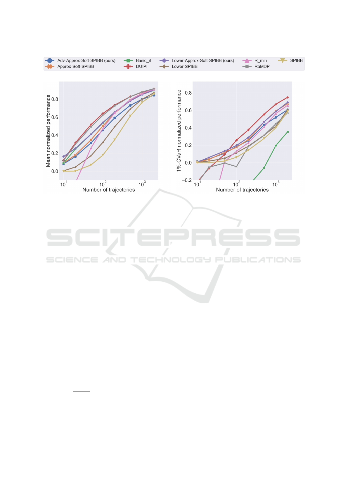
(a) Mean (b) 1%-CVaR

Figure 3: Mean (a) and 1%-CVaR (b) normalized performance over 10,000 trials on the Random MDPs benchmark for

= 0.9. In the context of SPI the focus lies on the 1%-CVaR. The mean performance is dominated by the algorithms

applying a penalty on the action-value function, while the restricting algorithms are winning for few data points in the risk-

sensitive 1%-CVaR measure and only lose to DUIPI in the long run. Among the SPIBB class, Lower-Approx-Soft-SPIBB

shows the best performance in both runs.

which gives a reward of 1. As the discount factor is

chosen as γ = 0.95, maximizing the return is equiva-

lent to ﬁnding the shortest route to the terminal state.

The baseline policy on each MDP is computed

such that its performance is approximately ρ

∗

(0) = ηV

∗

(0)+ (1 −η)V

∗

(0), where 0 ≤η ≤1

is the baseline performance target ratio interpolat-

ing between the performance of the optimal policy

∗

and the uniform policy π

. The generation of

the baseline policy starts with a softmax on the opti-

mal action-value function and continues with adding

random noise to it, until the desired performance is

achieved (Nadjahi et al., 2019). To counter the ef-

fects from incorporating knowledge about the opti-

mal policy, the MDP is altered after the generation of

the baseline policy by transforming one regular state

to a terminal one, called good easter egg, which also

yields a reward of 1.

In this experiment, 10, 000 iterations were run

and the performances are normalized to make them

more comparable between different runs by calcu-

lating

−ρ

∗

−ρ

. Thus,

< 0 means a worse

performance than the baseline policy,

> 0 means

an improvement w.r.t. the baseline policy and

= 1

means the optimal performance was reached. As we

are interested in Safe Policy Improvement, we follow

Chow et al. (2015), Laroche et al. (2019), and Nad-

jahi et al. (2019) and consider besides the mean per-

formance also the 1%-CVaR (Critical Value at Risk)

performance, which is the mean performance over the

1% worst runs.

These two measures can be seen in Figure 3,

where we show the performance of the algorithms for

their optimal respective hyper-parameter, as displayed

in Table 1. In the mean performance, RaMDP and

DUIPI outperform every other algorithm as soon as at

least 20 trajectories are observed. They are followed

by Lower-Approx-Soft-SPIBB and Basic RL, which

come just before the other Soft-SPIBB algorithms.

Approx-Soft-SPIBB shows a slightly better perfor-

mance than its successor Adv-Approx-Soft-SPIBB.

-SPIBB (SPIBB) and Π

≤b

-SPIBB (Lower-SPIBB)

seem to perform the worst. While R-MIN exhibits is-

sues when the data set is very small, it catches up with

the others for bigger data sets. Interestingly, Basic

RL performs generally quite well, but is still outper-

formed by some algorithms, which might be surpris-

ing as the others are intended for safe RL instead of

an optimization of their mean performance. The rea-

son for this might be that considering the uncertainty

of the action-value function is even beneﬁcial for the

mean performance.

The performance in the worst percentile looks

ICAART 2022 - 14th International Conference on Agents and Artiﬁcial Intelligence

148

very different. Here, it can be seen how well the safety

mechanisms of some of the algorithms work, par-

ticularly when compared to Basic RL, which shows

the worst overall 1%-CVaR performance. Also, R-

MIN and RaMDP perform very poorly especially for

a low number of trajectories. For less than 100 tra-

jectories, DUIPI performs also very poorly but out-

performs every other algorithm for bigger data sets.

An interesting observation is that all the SPIBB and

Soft-SPIBB algorithms perform in the beginning ex-

tremely well, which is expected as they fall back

to the behavior policy if not much data is available.

The ranking in the SPIBB family stays the same

for the 1%-CVaR as it has been for the mean per-

formance: Lower-Approx-Soft-SPIBB performs the

best, closely followed ﬁrst by Approx-Soft-SPIBB

and Adv-Approx-Soft-SPIBB. Π

≤b

-SPIBB falls a bit

behind but still manages to perform better than the

original Π

-SPIBB.

5.2 Wet Chicken Benchmark

Besides reproducing the results of Nadjahi et al.

(2019) for additional algorithms, we extend their ex-

periments to a more realistic scenario for which we

have chosen the discrete version of the Wet Chicken

benchmark (Hans and Udluft, 2009) because of its

heterogeneous stochasticity. Figure 4 visualizes the

setting of the Wet Chicken benchmark. The basic

idea behind it is that a person ﬂoats in a small boat

on a river. The river has a waterfall at one end and the

goal of the person is to stay as close to the waterfall

as possible without falling down. Thus, the closer the

person is to the waterfall the higher the reward gets,

but upon falling down they start again at the starting

place, which is as far away from the waterfall as pos-

sible. Therefore, this is modeled as a non-episodic

MDP.

The whole river has a length and width of 5, so,

there are 25 states. The starting point is (x, y) = (0, 0)

and the waterfall is at x = 5. The position of the

person at time t is denoted by the pair (x

, y

). The

river itself has a turbulence which is stronger near the

shore the person starts close to (y = 0) and a stream

towards the waterfall which is stronger near the other

shore (y = 4). The velocity of the stream is deﬁned as

= y

and the turbulence as b

= 3.5−v

. The effect

of the turbulence is stochastic; so, let τ

∼U(−1, 1)

be the parameter describing the stochasticity of the

turbulence at time t.

The person has 5 actions, which are (a

and a

describe the inﬂuence of an action on x

and y

, re-

spectively):

• Drift: The person does nothing, in formula

Figure 4: The setting of the Wet Chicken benchmark used

for reinforcement learning. The boat starts at (x, y) = (0, 0)

and starts there again upon falling down the waterfall at x =

5. The arrows show the direction and strength of the stream

towards the waterfall. Additionally, there are turbulences

which are stronger for small y. The goal for the boat is

to stay as close as possible to the waterfall without falling

down.

, a

) = (0, 0).

• Hold: The person paddles back with half their

power, in formula (a

, a

) = (−1, 0).

• Paddle back: The person wholeheartedly paddles

back, in formula (a

, a

) = (−2, 0).

• Right: The person tries to go to the right parallel

to the waterfall, in formula (a

, a

) = (0, 1).

• Left: The person tries to go to the left parallel to

the waterfall, in formula (a

, a

) = (0, −1).

The new position of the person assuming no river

constraints is then calculated by

( ˆx, ˆy) = (round(x

+ a

+ v

+ τ

), round(x

+ a

))

(21)

where the round function is the usual one, i.e., a num-

ber is getting rounded down if the ﬁrst decimal is 4

or less and rounded up otherwise. Incorporating the

boundaries of the river yields the new position as

t+1



ˆx, if 0 ≤ ˆx ≤ 4

0, otherwise

(22)

and

t+1











0, if ˆx > 4

4, if ˆy > 4

0, if ˆy > 0

ˆy, otherwise

. (23)

As the aim of this experiment is to have a realistic

setting for Batch RL, we use a realistic behavior pol-

icy. Thus, we do not incorporate any knowledge about

the transition probabilities or the optimal policy as it

has been done for the Random MDPs benchmark. In-

stead we devise heuristically a policy, considering the

overall structure of the MDP.

Safe Policy Improvement Approaches on Discrete Markov Decision Processes

149

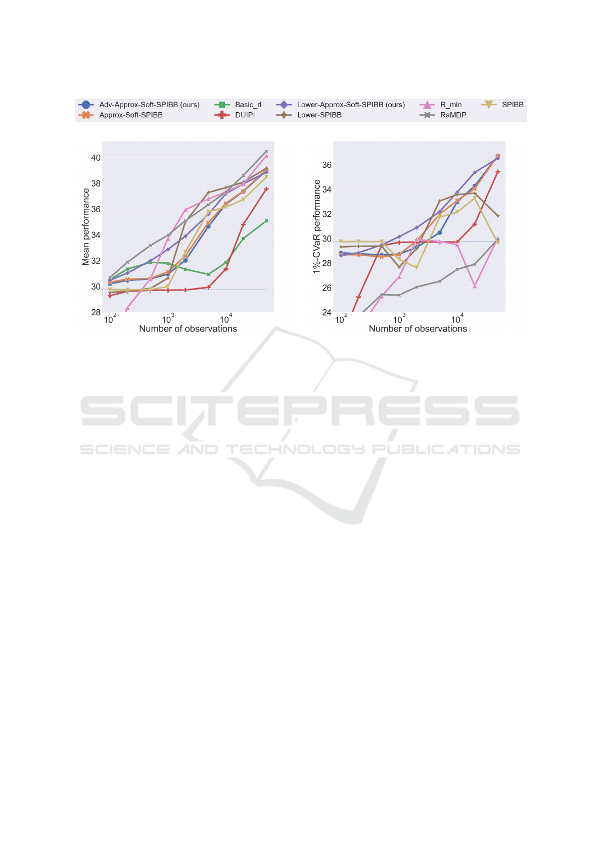
(a) Mean (b) 1%-CVaR

Figure 5: Mean (a) and 1%-CVaR (b) performance over 10,000 trials on the Wet Chicken benchmark for ε = 0.1 for the

baseline policy. The mean performance is dominated by RaMDP, while the restricting algorithms are winning in the risk-

sensitive 1%-CVaR measure. Among the SPIBB class, Lower-Approx-Soft-SPIBB shows the best performance in both runs.

Our behavior policy follows the idea that the most

beneﬁcial state might lie in the middle of the river at

(x, y) = (2, 2). This idea stems from two trade-offs.

The ﬁrst trade-off is between low rewards for a small

x and a high risk of falling down for a big x and the

second trade-off is between a high turbulence and low

velocity for a low y and the opposite for big y. To be

able to ensure the boat stays at the same place turbu-

lence and velocity should both be limited.

This idea is enforced through the following proce-

dure. If the boat is not in the state (2, 2), the person

tries to get there and if they are already there, they

use the action paddle back. Denote this policy with

′

. The problem with this policy is that it is deter-

ministic, i.e., in every state there is only one action

which is chosen with probability 1. This means that

for each state there is at most 1 action for which data

is available when observing this policy. This is coun-

tered by making π

′

ε-greedy, i.e., deﬁne the behavior

policy π

as the mixture

= (1 −ε)π

′

+ επ

(24)

where π

is the uniform policy which chooses every

action in every state with the same probability. ε was

chosen to be 0.1 in the following experiments.

Again, the experiment was run 10,000 times for

each algorithm and each hyper-parameter and show

the mean and 1%-CVaR performance in Figure 5 for

the optimal hyper-parameter, as displayed in Table 1.

Apart from DUIPI, the results are similar to those on

the Random MDPs benchmark. Again, the mean per-

formance of R-MIN is extremely bad for few data but

then improves strongly. Basic RL and DUIPI exhibit

the worst mean performance. All algorithms from the

SPIBB family perform very well, especially Lower-

Approx-Soft-SPIBB, and are only beaten by RaMDP.

Once more, the 1%-CVaR performance is of high

interest for us and Figure 5 conﬁrms many of the

observations from the Random MDPs benchmark as

well. We ﬁnd again that especially Basic RL—not

even visible in the plot due to its inferior perfor-

mance—, but also RaMDP and R-MIN have prob-

lems competing with the SPIBB and Soft-SPIBB al-

gorithms. Overall, Lower-Approx-Soft-SPIBB per-

forms the best, followed by Adv-Approx-Soft-SPIBB

and Approx-Soft-SPIBB.

These two experiments demonstrate that restrict-

ing the set of policies instead of adjusting the action-

value function can be very beneﬁcial for the safety as-

pect of RL, especially in complex environments and

for a low number of observations. On the contrary,

from a pure mean performance point of view it is fa-

vorable to rather adjust the action-value function.

ICAART 2022 - 14th International Conference on Agents and Artiﬁcial Intelligence

150

6 CONCLUSION

We show that the algorithms proposed in Nadjahi

et al. (2019) are not provably safe and propose a new

version that is provably safe. We also adapt their ideas

to derive a heuristic algorithm which shows, among

the entire SPIBB class on two different benchmarks,

both the best mean performance and the best 1%-

CVaR performance, which is important for safety-

critical applications. Furthermore, it proves to be

competitive in the mean performance against other

state of the art uncertainty incorporating algorithms

and especially to outperform them in the 1%-CVaR

performance. Additionally, it has been shown that

the theoretically supported Adv-Approx-Soft-SPIBB

performs almost as well as its predecessor Approx-

Soft-SPIBB, only falling slightly behind in the mean

performance.

The experiments also demonstrate different prop-

erties of the two classes of SPI algorithms in Figure 1:

algorithms penalizing the action-value functions tend

to perform better in the mean, but lack in the 1%-

CVaR, especially if the available data is scarce.

Perhaps the most relevant direction of future work

is how to apply this framework to continuous MDPs,

which has so far been explored by Nadjahi et al.

(2019) without theoretical safety guarantees. Apart

from theory, we hope that our observations of the two

classes of SPI algorithms can contribute to the choice

of algorithms for the continuous case.

REFERENCES

Brafman, R. I. and Tennenholtz, M. (2003). R-MAX - a

general polynomial time algorithm for near-optimal

reinforcement learning. Journal of Machine Learning

Research, 3.

Chow, Y., Tamar, A., Mannor, S., and Pavone, M. (2015).

Risk-sensitive and robust decision-making: a CVaR

optimization approach. In Proceedings of the 28th

International Conference on Neural Information Pro-

cessing Systems.

Dantzig, G. B. (1963). Linear Programming and Exten-

sions. RAND Corporation, Santa Monica, CA.

Fujimoto, S., Meger, D., and Precup, D. (2019). Off-policy

deep reinforcement learning without exploration. In

Proc. of the 36th International Conference on Ma-

chine Learning.

Garc

ıa, J. and Fernandez, F. (2015). A Comprehensive Sur-

vey on Safe Reinforcement Learning. Journal of Ma-

chine Learning Research., 16.

Hans, A., Duell, S., and Udluft, S. (2011). Agent self-

assessment: Determining policy quality without ex-

ecution. In IEEE Symposium on Adaptive Dynamic

Programming and Reinforcement Learning.

Hans, A. and Udluft, S. (2009). Efﬁcient Uncertainty Propa-

gation for Reinforcement Learning with Limited Data.

In Artiﬁcial Neural Networks – ICANN, volume 5768.

Lange, S., Gabel, T., and Riedmiller, M. (2012). Batch

Reinforcement Learning. In Reinforcement Learning:

State-of-the-Art, Adaptation, Learning, and Optimiza-

tion. Springer, Berlin, Heidelberg.

Laroche, R., Trichelair, P., and Tachet des Combes, R.

(2019). Safe policy improvement with baseline boot-

strapping. In Proc. of the 36th International Confer-

ence on Machine Learning.

Leurent, E. (2020). Safe and Efﬁcient Reinforcement Learn-

ing for Behavioural Planning in Autonomous Driving.

Theses, Universit

e de Lille.

Levine, S., Kumar, A., Tucker, G., and Fu, J. (2020). Ofﬂine

reinforcement learning: Tutorial, review, and perspec-

tives on open problems. CoRR, abs/2005.01643.

Nadjahi, K., Laroche, R., and Tachet des Combes, R.

(2019). Safe policy improvement with soft baseline

bootstrapping. In Proc. of the 2019 European Confer-

ence on Machine Learning and Principles and Prac-

tice of Knowledge Discovery in Databases.

Nilim, A. and El Ghaoui, L. (2003). Robustness in Markov

decision problems with uncertain transition matrices.

In Proc. of the 16th International Conference on Neu-

ral Information Processing Systems.

Petrik, M., Ghavamzadeh, M., and Chow, Y. (2016). Safe

policy improvement by minimizing robust baseline re-

gret. In Proceedings of the 30th International Con-

ference on Neural Information Processing Systems,

NIPS’16, Red Hook, NY, USA. Curran Associates

Inc.

Schaefer, A. M., Schneegass, D., Sterzing, V., and Udluft, S.

(2007). A neural reinforcement learning approach to

gas turbine control. In International Joint Conference

on Neural Networks.

Schneegass, D., Hans, A., and Udluft, S. (2010). Uncer-

tainty in Reinforcement Learning - Awareness, Quan-

tisation, and Control. In Robot Learning. Sciyo.

Scholl, P. (2021). Evaluation of safe policy improvement

with soft baseline bootstrapping. Master’s thesis,

Technical University of Munich.

Sim

ao, T. D., Laroche, R., and Tachet des Combes, R.

(2020). Safe Policy Improvement with an Estimated

Baseline Policy. In Proc. of the 19th International

Conference on Autonomous Agents and MultiAgent

Systems.

Sutton, R. S. and Barto, A. G. (2018). Reinforcement learn-

ing: An introduction. MIT press.

Thomas, P. S. (2015). Safe Reinforcement Learning. Doc-

toral dissertations., University of Massachusetts.

Wang, R., Foster, D., and Kakade, S. M. (2021). What

are the statistical limits of ofﬂine RL with linear func-

tion approximation? In International Conference on

Learning Representations.

Safe Policy Improvement Approaches on Discrete Markov Decision Processes

151