Unsupervised Learning of State Representation using Balanced View

Spatial Deep InfoMax: Evaluation on Atari Games

Menore Tekeba Mengistu

1,2

, Getachew Alemu

, Pierre Chevaillier

and Pierre De Loor

School of Electrical and Computer Engineering, Addis Ababa University, King George VI Street, Addis Ababa, Ethiopia

Lab-STICC, UMR CNRS 6285, ENIB, France

Keywords:

Unsupervised Learning, Autonomous Agents, State Representation Learning, Contrastive Learning,

Atari Games.

Abstract:

In this paper, we present an unsupervised state representation learning of spatio-temporally evolving sequences

of autonomous agents’ observations. Our method uses contrastive learning through mutual information (MI)

maximization between a sample and the views derived through selection of pixels from the sample and other

randomly selected negative samples. Our method employs balancing MI by ﬁnding the optimal ratios of

positive-to-negative pixels in these derived (constructed) views. We performed several experiments and de-

termined the optimal ratios of positive-to-negative signals to balance the MI between a given sample and the

constructed views. The newly introduced method is named as Balanced View Spatial Deep InfoMax (BVS-

DIM). We evaluated our method on Atari games and performed comparisons with the state-of-the-art unsuper-

vised state representation learning baseline method. We show that our solution enables to successfully learn

state representations from sparsely sampled or randomly shufﬂed observations. Our BVS-DIM method also

marginally enhances the representation powers of encoders to capture high-level latent factors of the agents’

observations when compared with the baseline method.

1 INTRODUCTION

Self learning of sensory data are considered as a fun-

damental cognitive capability of animals and spe-

cially humans (Marr, 1982; Gordon and Irwin, 1996).

Therefore, it is important to endow autonomous artiﬁ-

cial agents with such cognitive capability (Nair et al.,

2018; Lake et al., 2017). Currently, it is possible

to train a model through supervised learning, from

raw sensory data with machine learning architectures

(Khan et al., 2020). However, this raises some difﬁ-

culties: the need of huge databases that must be la-

belled (Russakovsky et al., 2015), the time required

to train the model but more fundamentally, the differ-

ence with the way living beings are able to learn by

themselves to recognize shapes, without the need of

million of annotated samples. Consequently, some re-

searchers have adopted another way, closer to natural

or psychological observations. For instance (Forestier

et al., 2017; P

e et al., 2018) used intrinsically mo-

tivated exploration and unsupervised learning princi-

ples to give an agent the capability to acquire new

knowledge and skills. The key principle of unsuper-

vised learning is to compare different perceptions of a

same context and to ﬁnd out what distinguishes them

(Bachman et al., 2019; Oord et al., 2018). However,

modeling high-level representation from raw sensory

data through unsupervised learning remains challeng-

ing and is far to be as efﬁcient as supervised learning.

To compare algorithms, benchmark based on

Atari 2600 games (Bellemare et al., 2013) are gener-

ally used because they endow state variables (location

of the player, location of different items, etc.) which

are generative factors of the images. This state vari-

ables are representations accessible from the source

code of the game and can be learned. Moreover, there

are several Atari games of diverse natures and number

of state variables with varied conditions of the envi-

ronment. Thus it allows to collect enough samples

for each game and to carry out evaluations across sev-

eral games to assess the generalization capability of

the learning method. For this task, and to our knowl-

edge, the Spatio-Temporal Deep InfoMax (ST-DIM)

(Anand et al., 2019) is the state-of-the-art baseline.

In this work, we have introduced a new ap-

proach for unsupervised state representation learning

of spatio-temporally evolving data sequences based

on maximizing contrastive Mutual Information (MI).

110

Mengistu, M., Alemu, G., Chevaillier, P. and De Loor, P.

Unsupervised Learning of State Representation using Balanced View Spatial Deep InfoMax: Evaluation on Atari Games.

DOI: 10.5220/0010785000003116

In Proceedings of the 14th International Conference on Agents and Artiﬁcial Intelligence (ICAART 2022) - Volume 2, pages 110-119

ISBN: 978-989-758-547-0; ISSN: 2184-433X

Our method is known as Balanced View Spatial Deep-

InfoMax (BVS-DIM). The learning of BVS-DIM de-

pends on maximizing MI between the whole fea-

tures of an image and the features of the patches of

its views; and maximizing MI between the features

of the patches of the image and the corresponding

patches of its views. Since these MI maximization

correspondences of the global and local features is

in spatial axes, we used the term ”Spatial”. We bal-

ance the ratio of pixels taken from the sample itself

and from other samples in the constructed views and

hence, we used the term ”Balanced View”.

Our method is proposed to enable autonomous

agents’ unsupervised learning from sparsely or irreg-

ularly sampled observations or observations with no

time stamp at all. As discussed in section 3, these

scenarios of learning are unaddressed by ST-DIM,

which success strongly depends on consecutive time

step samples with high sampling rates.

In section 2, we discussed the related works and in

section 3 we presented the motivation of this research

work. Then in section 4, we detailed our method,

BVS-DIM. In section 5, we described the experimen-

tal settings. Then in section 6, it is our results and

discussion section. We compared our results with the

state-of-the-art ST-DIM method and other methods

with different ways to create positive views. In con-

clusion (section 7), we show how BVS-DIM achieved

the objectives we set in section 3 with performances

exceeding the baseline.

2 RELATED WORKS

In state representation learning, current unsupervised

methods use three approaches: generative decoding

of the data using Variational Auto Encoders (VAEs),

generative decoding of the data using prediction in

pixel-space (prediction of future frames in videos and

video games (Oh et al., 2015)) and scalable estimation

of mutual information (MI) between the input and the

output. The scalability of the MI based representation

is both in dimensions, sample size and with a char-

acteristic of achieving good performance in different

settings (Belghazi et al., 2018). However, the gen-

erative models using VAEs or predictive pixels tend

to capture pixel level details rather than abstract la-

tent factors. The generative decoding aims in recon-

structing the input image with pixel level reconstruc-

tion accuracy (Kingma and Welling, 2013; Sønderby

et al., 2016). On the other hand, representation learn-

ing based on maximizing MI focuses on enhancing

MI either between representations of different views

of the same sample or between an input and its repre-

sentation. This objective of maximizing MI helps to

learn semantically meaningful and interpretable (dis-

entangled) representations (Chen et al., 2016) and en-

ables to have better representation of a given sample’s

overall feature rather than local and low-level details.

Unsupervised Representation Learning: Recent

works on unsupervised representation learning extract

latent representations by maximizing a lower bound

on the mutual information between the representation

and the input. DIM (Hjelm et al., 2019) performs

unsupervised learning of representations by maximiz-

ing the Jensen-Shannon (JD) divergence between the

joint and product of marginals of an image and its

patches. DIM’s representation learning also works

well with loss based on Noise Contrastive Estimation

(InfoNCE) (Oord et al., 2018) and Mutual Informa-

tion Neural Estimation (MINE) (Belghazi et al., 2018)

in addition to JD. Another similar work with DIM

(Bachman et al., 2019) uses representations learned

through maximizing the MI between a given image

and its augmented views. See (Poole et al., 2019)

and (Anand et al., 2019) for more details on repre-

sentation learning through MI maximization between

inputs and outputs.

State Representation Learning: Learning state

representations is an active area of research within

robotics and reinforcement learning (Nair et al., 2018;

e et al., 2018). Most existing state representation

learning methods are based on handcrafted features

and/or through supervised training using labelled data

(Jonschkowski and Brock, 2015; Jonschkowski et al.,

2017; Lesort et al., 2018). However, agents and robots

can’t learn from new observations when they are ex-

posed to new and unseen environments. Therefore,

most recent unsupervised state representations were

introduced like TCN (Sermanet et al., 2018), TDC

(Ma and Collins, 2018) and more recently, ST-DIM

(Anand et al., 2019), which is the state-of-the-art

baseline to our BVS-DIM method. Our BVS-DIM is

also based on DIM (Hjelm et al., 2019). ST-DIM used

Atari games for evaluating their learning of state rep-

resentations. The state variables of the Atari games

are the controllers of the game dynamics and the de-

tails of these state variables are provided in (Anand

et al., 2019).

Our work is closely related to DIM (Hjelm et al.,

2019), AMDIM (Bachman et al., 2019) and ST-DIM

(Anand et al., 2019) even though the ﬁrst two are gen-

eral purpose representation learning methods tested

on real-world data-sets such as ImageNet (Deng et al.,

2009).

Unsupervised Learning of State Representation using Balanced View Spatial Deep InfoMax: Evaluation on Atari Games

111

3 MOTIVATION

An autonomous agent should be capable of learning

in an unsupervised way. ST-DIM is an unsupervised

state representation learning from visual observations.

However, the learning method of ST-DIM depends on

the consecutive time step visual observations (Anand

et al., 2019). Hence ST-DIM has the following limi-

tations.

1. Sampling Rate: The learning of ST-DIM only

depends on the consecutive time samples. These

consecutive samples are similar with each-other

due to high sampling rates and one can be con-

sidered as the view of the other. Agents may have

sparse sampling rates and may not collect samples

frequently. In this case, consecutive time samples

wouldn’t be similar and hence, the ST-DIM ap-

proach can’t be appropriate enough to capture the

latent generative factors of the environment.

2. Selective Sample Collection: Autonomous

learning from a one time collected dataset makes

the autonomous agent limited to the environment

from which the samples are collected. To extend

the learning across longer time and diverse envi-

ronments, agents may learn while they are collect-

ing samples and make replacements of samples

with new relevant experiences using some selec-

tion criteria when their memory is full. In this

case, the collected datasets won’t be consecutive

time step; the sampling frequency won’t be uni-

form, or it may not have a time-stamp at all. In

such types of scenarios, ST-DIM approach can’t

be employed for the learning as it depends on the

similarity of consecutive samples.

To overcome these limitations, we proposed BVS-

DIM in which autonomous agents can learn from

data samples with randomly shufﬂed order, sparsely

sampled from the environment or time-consecutive as

well. Our BVS-DIM method is inspired by different

biological and computational research ﬁndings and

combined them to create a better state representation

learning method. We adopted the concept of hard-

mixture of features from (Kalantidis et al., 2020), the

concept of both positive and negative samples for bet-

ter learning from (Carlson et al., 2014) and (Visani

et al., 2020), the concept of contrastive relations of a

pixel in a given image to the pixels of the entire im-

ages in the data-set from (Wang et al., 2021) and the

concept of data augmentation from (Bachman et al.,

2019). We created constructed views of a given sam-

ple by selecting pixels from itself (positive signals)

and pixels from another sample randomly selected

from the same mini-batch (negative signals). We used

MI maximization between learned representations of

a sample and its constructed views.

The objective of our BVS-DIM method is to learn

features with latent factors of the agents’ observation

even under the absence of signiﬁcant similarity be-

tween time consecutive samples or randomly shuf-

ﬂed samples of autonomous agents. It enables the

autonomous agent to capture every spatially evolv-

ing factor including controllable ones and the envi-

ronment such as state variables. We have made the

following contributions.

1. We devised a new unsupervised state represen-

tation learning method that can learn from sam-

ples collected by autonomous agents regardless of

their chronological order and sampling rate.

2. We achieved marginally better result when com-

pared to ST-DIM, the state of the art baseline

method, both for time-consecutive and randomly

shufﬂed collected samples.

4 BALANCED VIEW SPATIAL

DEEP INFOMAX

The core idea of our BVS-DIM method is in creat-

ing balanced views of a given sample using selec-

tion methods of pixels from itself and pixels from

other randomly selected sample of the same mini-

batch. Balanced view is created through selection

of the ratio of positive-to-negative signals in the con-

structed view. Our method extends the state represen-

tation power of spatio-temporally evolving sequences

of data by letting the encoder capture the discrimi-

native features from the mixed positive and negative

signals exploiting both similarity and contrast in a sin-

gle constructed view of a given sample. Here after

we used ”positive sample” to refer to a given anchor

sample itself, ”negative sample” to refer to any other

sample randomly drawn from the same mini-batch.

We assumed a setting where an agent interacts

with its environment and observes high-dimensional

observations across several episodes and we formed

two sample sets from these episodes. The ﬁrst set

of observations preserving their temporal ordering

is given as χ = {x

, x

, ..., x

}. The second set

of observations being randomly shufﬂed is given as

′

= {x

′

, x

′

, x

′

, ..., x

′

Taking the advantage of the success of ST-DIM,

where the frames of consecutive time-steps x

and

t+1

are similar with each other, these consecutive

frames are taken as the view of one another. How-

ever, learning in ST-DIM is limited to time sequenced

samples, and we hypothesize the success of state rep-

ICAART 2022 - 14th International Conference on Agents and Artiﬁcial Intelligence

112

resentation learning in ST-DIM depends on the sim-

ilarity factor of consecutive observations. When the

sampling rates of the observations are more frequent,

the consecutive frames will have high similarity and

vice-versa. Let us assume that we have a positive an-

chor sample x

and two other randomly selected neg-

ative samples x

∗

and x

∗

uniformly sampled from χ or

′

. We shall construct two positive views x

min

and

max

from (x

, x

∗

) and (x

, x

∗

) pairs using the fol-

lowing simple min and max pixel-wise operations, re-

spectively.

min

(i, j) := min(x

(i, j), x

∗

(i, j)) (1)

max

(i, j) := max(x

(i, j), x

∗

(i, j)) (2)

The positive sample probably has 50% signal con-

tribution in x

min

and x

max

constructed views. How-

ever, the balancing ratios in the newly constructed

views affect the representation learning performance.

Our prime purpose is to balance the ratio of positive-

to-negative signals in these constructed views. Let

p represent the probability of assigning the pixel

of x

bmn

and x

bmx

from pixels of x

modifying con-

structed views of x

min

and x

max

. To increase the ra-

tio of positive-to-negative signals from 0.5 to some

r where r > 0.5, we shall assign the value of p as

p = 2 ∗ (r − 0.5). Then the new ﬁnally modiﬁed con-

structed views x

bmn

and x

bmx

is given by equations

4 and 5, respectively. Let R be an array of normal

(Gaussian) distribution with center p in range [0, 1]

and C be a Boolean array. Both R and C have the

same dimension as x

and equation 3 initializes the

Boolean array C.

i, j



true

if R

i, j

< p

f alse

otherwise

(3)

bmn

(i, j) :=



(i, j)

if C

i, j

= true

min

(i, j)

otherwise

(4)

bmx

(i, j) :=



(i, j)

if C

i, j

= true

max

(i, j)

otherwise

(5)

4.1 Maximizing Mutual Information

across Balanced Views

Similar to ST-DIM, we used two types of MI esti-

mations. The ﬁrst is global-to-local (GL) where the

MI between the global (whole) features of a sample

and the features of local patches of its views are com-

puted. The second one is local-to-local (LL) where

the MI between the features of local patches of the

sample and its corresponding views are estimated.

The combination of these two MI estimations is de-

noted as GL-LL. Therefore, our BVS-DIM is used

with either the GL-LL or GL-only MI objective for

both time-sequenced and randomly selected tuples of

samples. Then we used MI maximization function

between a sample and its constructed views to en-

hance representation learning. We hypothesize that

such enhancement of representation learning is possi-

ble through balancing the ratio of positive-to-negative

signals in the constructed views.

For a given MI estimator, we used the GL objec-

tive in equation 7 to maximize the MI between global

features of x

and features of small patches of x

bmn

and x

bmx

. The Local-Local (LL) objective in equa-

tion 8 maximizes MI between the local feature of x

with the corresponding local feature of x

bmn

and x

bmx

The LL MI objective is used in combination with GL

MI objective as GL-LL. The views, x

bmn

and x

bmx

, are

constructed as mixed pixels from the positive sample

and two negative samples, (x

∗

or x

∗

which are se-

lected in a uniformly random way as given in equa-

tions 1 through 5). We have used the GL MI objective

alone as well as the combined GL-LL MI objective in

our tests. Figure 1 represents a visual depiction of our

model, BVS-DIM.

We used InfoNCE (Oord et al., 2018) as MI es-

timator, a multi-sample variant of noise-contrastive

estimation (NCE) (Gutmann and Hyv

arinen, 2010).

This MI estimator worked well with DIM and ST-

DIM along with GL and GL-LL objectives, respec-

tively. Let {(x

, y

)}

i=1

be a paired dataset of N sam-

ples from some joint distribution p(x, y). We consider

any sample i of (x

, y

) from this joint p(x, y) are the

positive sample pairs and any i ̸= j of (x

, y

) are neg-

ative sample pairs. InfoNCE objective uses a score

function f (x, y) which assigns larger values to posi-

tive sample pairs and smaller values to negative sam-

ple pairs by maximizing equation 6 as discussed in

details on (Oord et al., 2018) and (Poole et al., 2019).

NCE

({(x

, y

)}

i=1

) =

∑

i=1

log

exp( f (x

, y

))

∑

j=1

exp( f (x

, y

))

(6)

The MI objective function given in equation 6 has

also been referred to as multi-class n-pair loss (Sohn,

2016), (Sermanet et al., 2018), ranking-based NCE

(Ma and Collins, 2018) and is similar to MINE (Bel-

ghazi et al., 2018) and the JSD-variant of DIM (Hjelm

et al., 2019).

For fair comparison of our model with ST-DIM,

we have used a bilinear model W for the score func-

tion f (x, y) = ψ(x)

W ψ(y), where ψ is our represen-

tation encoder. The bi-linear model in combination

with InfoNCE enables the encoder to learn linearly

predictable representations and helps in learning rep-

resentations at the semantic level (Anand et al., 2019).

Let X

= {(x

, x

∗

, x

∗

}

i=1

be a mini-batch of ran-

domly selected tuples of samples from χ

′

. We con-

Unsupervised Learning of State Representation using Balanced View Spatial Deep InfoMax: Evaluation on Atari Games

113

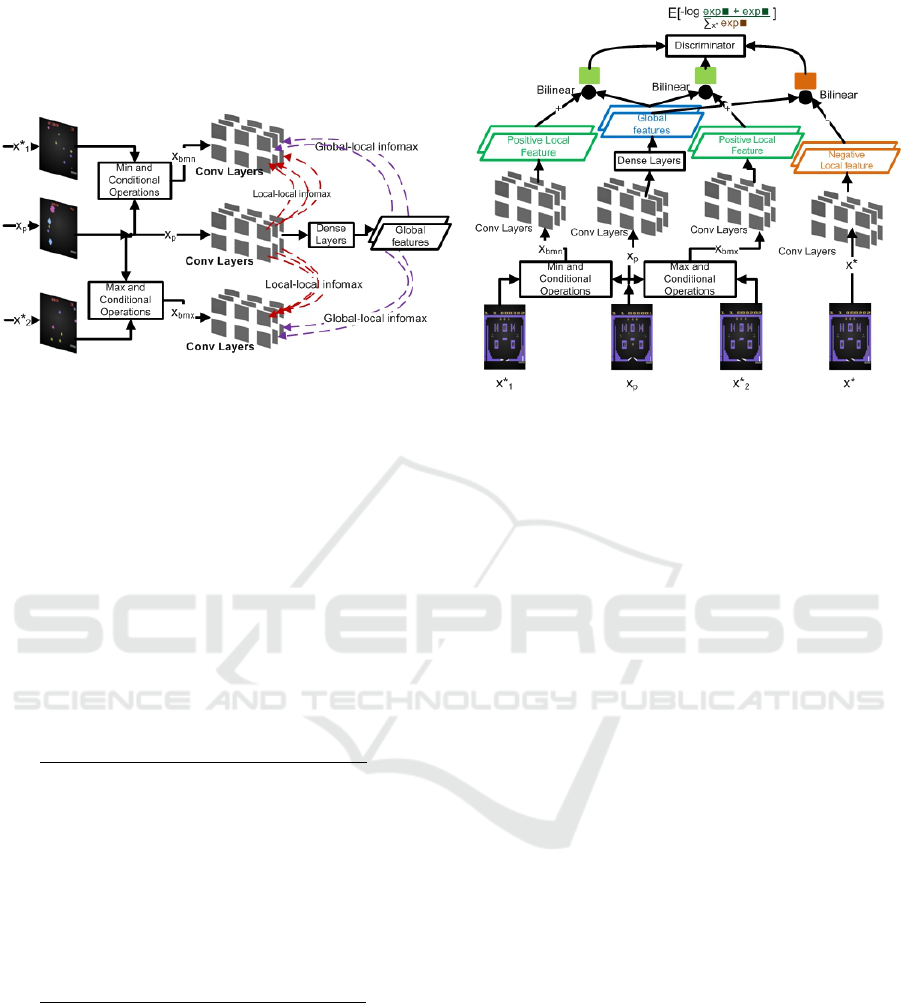
Figure 1: A schematic overview of Balanced View Spatial Deep InfoMax (BVS-DIM). Left: The two different mutual in-

formation objectives i.e. Local-Local (LL) infomax and Global-Local (GL) infomax. Right: A simpliﬁed version of the GL

contrastive task. The two negative samples x

∗

and x

∗

represent negative samples selected from the mini-batch randomly with

uniform probability distributions. These two negative samples are used along x

to construct the x

bmn

and x

bmx

balanced

views. x

∗

represents all negative samples in the mini-batch including x

∗

and x

∗

, and other than x

. In practice, we used only

two positive samples and multiple negative samples.

struct two loss functions modifying the generic In-

foNCE equation 6 for our BVS-DIM: the loss follow-

ing the GL MI objective, L

, as given in equation 7

and the loss following the LL MI objective, L

, as

given in equation 8.

∑

m=1

∑

n=1

−log

exp(g

m,n

, x

bmn

)) + exp(g

m,n

, x

bmx

))

(

∑

∗

∈X and x

∗

̸=x

exp(g

m,n

, x

∗

)))

(7)

where the score function for the GL MI objective,

m,n

, x

) = ψ(x

)

m,n

) and ψ

m,n

is the lo-

cal feature vector produced by an intermediate layer

in ψ at the (m, n) spatial location.

∑

m=1

∑

n=1

−log

exp( f

m,n

, x

bmn

)) + exp( f

m,n

, x

bmx

))

∑

∗

∈Xandx

∗

̸=x

exp( f

m,n

, x

∗

)))

(8)

where the score function for the LL MI objective,

m,n

, x

) = ψ

m,n

)

m,n

5 EXPERIMENTAL SETUP

Even though unsupervised learning of state represen-

tations are developed, evaluating the usefulness of a

representation is still an open problem because the

objectives and core utilities of these features during

training are different when used in their downstream

tasks. For example, measuring classiﬁcation perfor-

mance will only show the goodness of the represen-

tation for class relevant features. Devising a generic

way of measurement of the general goodness of the

representation is essential (Anand et al., 2019).

Video games, like Atari games, are useful candi-

date for evaluating visual representation learning al-

gorithms and they provide ready access to the under-

lying ground truth states which are required to evalu-

ate performance of different techniques. In ST-DIM,

the ground truth state information (a state label for

every example frame generated from the game) has

been annotated for each frame of 22 Atari games to

make evaluation of the goodness of the representa-

tion (See (Anand et al., 2019)). We have used this

ST-DIM benchmark on Atari games using the Ar-

cade Learning Environment (ALE) (Bellemare et al.,

2013) and modiﬁed it to incorporate theBVS-DIM

method for evaluating the goodness of the learned

representations. Therefore, the goodness of the rep-

resentations is evaluated against the performance of

bi-linear classiﬁers for state variables taking the fea-

tures learned as an input. There are categories of state

variables, and the classiﬁcation performances are av-

eraged for each category in each game. Then ﬁnal

average of the game across categories is reported as

F1 classiﬁcation score of the game. For the sake

of comparison, we have used the same data collec-

tion methods and the same randomly-initialized CNN

ICAART 2022 - 14th International Conference on Agents and Artiﬁcial Intelligence

114

encoder (RANDOM-CNN) architecture taken from

(Mnih et al., 2013) and adapted for the full 160x210

Atari frame size with the feature representation space

of 256.

In probing stage, we trained the 256-way linear

classiﬁer models with the learned representation of

the encoder as input. Only state variables with high

entropy are considered, and duplicates are removed.

We used the same probing conditions, number of

training, validation and testing samples as well as

early stopping and a learning rate scheduler as used

in ST-DIM.

We made two categories of tests. The ﬁrst

category, for consecutive time step tuples of

t−1

, x

t+1

) from χ. For this category, we have

used equations 1 and 2 to construct the views x

min

and

max

from (x

t−1

, x

) and (x

, x

t+1

), respectively. We

have used GL-only MI objective. For the second cat-

egory of tests, we have used randomly selected tuples

of (x

, x

∗

, x

∗

) from χ

′

. We have followed the opera-

tions speciﬁed in equations 1 through 5 to construct

the views x

bmn

and x

bmx

from (x

, x

∗

) and (x

, x

∗

), re-

spectively. We tested several balancing ratios rang-

ing from 0.65 to 0.85 with the interval of signiﬁcant

change, i.e. 0.05. We also tested both for the GL-only

and the combined GL-LL MI objectives.

Since number of tests were in the order of hun-

dreds for the second category, we limited the num-

ber of epochs and for fair comparison, the bench-

mark tests are also re-executed. To balance the ra-

tio of positive-to-negative signals in the constructed

views, we performed the tests on ﬁve Atari games

with ratios of {0.65, 0.70, 0.75, 0.80, 0.85} for both

GL-only and GL-LL MI objectives. From these ﬁve

game experiments, we found 0.70 and 0.75 for GL-

only and 0.80 for GL-LL MI objectives to work well

in the goodness of the learned state representations.

Based on the results, we performed tests for all 22

Atari games for GL-only-0.70, GL-only-0.75 and GL-

LL-0.80 along with the benchmark, ST-DIM, method

and made comparisons. To show how ST-DIM also

works for randomly selected pairs, we made two sets

of tests for ST-DIM; ST-DIM (C) stands for ST-DIM

with consecutive (t and t +1) observations while ST-

DIM (R) stands for ST-DIM with randomly selected

pairs of observations selected from the mini-batch

with uniform probability distribution. To make com-

parisons with contrastive learning based on other aug-

mented views, we made tests using views created as

in AMDIM (Bachman et al., 2019). We also made

tests replacing random noise instead of taking pixels

from negative samples for constructed views in the

mini-batch (BVS-DIM with noise).

Additionally, we have made ablation analysis by

making a breakdown of the results with respect to

each category of state variables. We have also made

a test on the presence of an easy to exploit features,

bounding boxes on each display variables, and made

comparison with the baseline method.

6 RESULTS AND DISCUSSION

As presented in section 4, the goodness of the repre-

sentation is its capability in capturing the underlying

generative factors of the environment. In Atari games,

the crucial underlying generative factors of the envi-

ronment are state variables which can be directly used

to control the game dynamics or query the game infor-

mation (Bellemare et al., 2013), (Anand et al., 2019).

6.1 Using Consecutive Time-step Tuples

As presented in section 5, consecutive time step

frames are used to create the constructed views (only

using equations 1 and 2) and used GL-only MI objec-

tive. We performed tests for the 22 Atari games with

NoFrameskip and 16 Atari Games with Framesskip

setting as well as the benchmark ST-DIM as shown

in Table 1. We have used GL-only MI objective and

achieved comparable results without applying balanc-

ing the positive-to-negative signal ratio as the frames

are consecutive.

With the 22 NoFrameskip Atari games, BVS-

DIM method outperformed ST-DIM in 12 games and

it has achieved almost comparable results with ST-

DIM in seven games. To show the robustness of

the BVS-DIM method under the absence of similar-

ity of consecutive observations, we tested the BVS-

DIM method and the benchmark with 16 Frameskip

type Atari games. The mean F1 classiﬁcation score

difference of the BVS-DIM method with ST-DIM

widened from 3% (with NoFrameskip games) to 5%

(with Frameskip games).

In the Frameskip setting, the BVS-DIM method

exceeded ST-DIM in 15 games while it has lev-

eled with ST-DIM in one game. The widened

gap observed between ST-DIM and BVS-DIM with

Frameskip games shows that the BVS-DIM method

is robust to the sampling rates of the observations

while ST-DIM is affected with the sampling rates of

the observations.

6.2 Using Randomly Selected Tuples

After constructing positive views x

bmn

and x

bmx

from

∗

, x

) and (x

, x

∗

), respectively using equations 1

through 5, we carry out tests for all 22 Atari games for

Unsupervised Learning of State Representation using Balanced View Spatial Deep InfoMax: Evaluation on Atari Games

115

Table 1: Probe F1 classiﬁcation scores averaged across categories for each game (data collected by random agents) with 2

and 3

columns for NoFrameskip and 4

and 5

columns for Frameskip = 4 setting. The GL-only MI objective with ratio

of 0.50 is used with BVS-DIM. Consecutive (t and t + 1) frames are used in both BVS-DIM and ST-DIM.

NoFrameskip Frameskip

GAME ST-DIM BVS-DIM (GL) ST-DIM BVS-DIM (GL)

ASTEROIDS 0.49 0.45 0.37 0.45

BERZERK 0.53 0.55 - -

BOWLING 0.96 0.96 0.95 0.98

BOXING 0.58 0.74 0.54 0.66

BREAKOUT 0.88 0.88 - -

DEMONATTACK 0.69 0.65 0.67 0.71

FREEWAY 0.81 0.95 0.76 0.87

FROSTBITE 0.75 0.76 - -

HERO 0.93 0.95 0.85 0.87

MONTEZUMAREVENGE 0.78 0.79 0.69 0.71

MSPACMAN 0.72 0.71 0.44 0.47

PITFALL 0.60 0.72 0.77 0.80

PONG 0.81 0.86 0.93 0.94

PRIVATEEYE 0.91 0.91 0.85 0.89

QBERT 0.73 0.67 - -

RIVERRAID 0.36 0.43 - -

SEAQUEST 0.67 0.72 - -

SPACEINVADERS 0.57 0.62 0.45 0.49

TENNIS 0.60 0.66 0.63 0.66

VENTURE 0.58 0.61 0.57 0.62

VIDEOPINBALL 0.61 0.66 0.53 0.55

YARSREVENGE 0.42 0.43 0.28 0.33

MEAN 0.68 0.71 0.64 0.69

GL-0.70, GL-0.75 and GL-LL-0.80 and made compar-

ison of BVS-DIM with ST-DIM.

The ST-DIM tests were re-executed as we

changed the number of epochs in this comparison and

we used 30 epochs for all tests of this category. Ta-

ble 2 shows the test results of the ST-DIM, GL-only

MI objective with 0.70 and 0.75 balancing ratios and

GL-LL MI objective with 0.80 balancing ratio. The

BVS-DIM with GL-LL MI objective and with 0.80

balancing ratio outperformed the benchmark ST-DIM

in 14 games while the baseline has exceeded in only

one game. To see the effect of negative sample pix-

els versus arbitrary noise in the constructed views, we

have modiﬁed the constructed views to take arbitrary

noise than taking pixels from negative samples. We

tested BVS-DIM with GL-LL-0.80 MI objective for

the noise (i.e. the noise constitutes about 20% in each

view) and we designate BVS-DIM-N (GL-LL-0.80)

in Table 2. The corresponding BVS-DIM (GL-LL-

0.80) with 20% pixels from other image samples has

a mean of 3% better performance than BVS-DIM-

N (GL-LL-0.80). This experiment shows that taking

pixels from other samples enhances the discriminat-

ing power of the encoders.

We have also made standard image augmentation

operation used as in AMDIM (Bachman et al., 2019)

and evaluated usign the same GL-LL MI objective

for fair comparison. The result of augmented views

contrastive learning using similar operators as used

in AMDIM for Atari games performs very low com-

pared to both BVS-DIM and ST-DIM. Even though

further analysis is required, we hypothesize that stan-

dard augmentation operators provided in AMDIM

(Bachman et al., 2019) aren’t optimal for state rep-

resentation learning of Atari games since the screen

images of Atari games contain smaller objects rele-

vant to the game outcome which may become much

distorted or lost in these augmentation operations.

The BVS-DIM method maintained the same per-

formance with randomly selected tuples and careful

selection of balancing ratio even with a training of

smaller number of epochs. The average F1 classiﬁca-

tion score of BVS-DIM with GL-only 0.70 exceeded

ST-DIM (C) (ST-DIM with consecutive frames) with

3% while the average F1 classiﬁcation score of BVS-

DIM with GL-LL 0.80 and GL-0.75 MI objectives at-

ICAART 2022 - 14th International Conference on Agents and Artiﬁcial Intelligence

116

Table 2: Probe F1 classiﬁcation scores averaged across categories for each game (data collected by random agents). The tuples

used in BVS-DIM methods are randomly selected from each mini-batch to construct two balanced views. The pairs used in

ST-DIM (R) are randomly selected pairs while the pairs used in ST-DIM (C) are time consecutive frames selected from each

mini-batch. We have included the results of the experimental results using the same image augmentation techniques as used

in AMDIM and the fully supervised learning for comparison.

GAME ST-

DIM

(R)

ST-

DIM

(C)

AM-

DIM

BVS-

DIM-N

(GL-LL

-0.80)

BVS-

DIM

(GL-

0.70)

BVS

-DIM

(GL-

0.75)

BVS

-DIM

(GL-LL

-0.80)

SU-

PER-

VISED

ASTEROIDS 0.41 0.48 0.34 0.45 0.46 0.45 0.48 0.52

BERZERK 0.30 0.51 0.43 0.53 0.54 0.56 0.56 0.68

BOWLING 0.34 0.94 0.60 0.86 0.95 0.94 0.93 0.95

BOXING 0.21 0.57 0.16 0.65 0.76 0.76 0.75 0.83

BREAKOUT 0.57 0.87 0.42 0.86 0.89 0.86 0.89 0.94

DEMONATTACK 0.44 0.69 0.30 0.65 0.66 0.64 0.66 0.83

FREEWAY 0.28 0.78 0.50 0.91 0.94 0.94 0.92 0.98

FROSTBITE 0.65 0.70 0.55 0.68 0.71 0.70 0.74 0.85

HERO 0.83 0.91 0.71 0.93 0.94 0.93 0.93 0.98

MONTEZUMAREVENGE 0.52 0.77 0.52 0.77 0.76 0.77 0.79 0.87

MSPACMAN 0.37 0.69 0.51 0.71 0.70 0.69 0.71 0.87

PITFALL 0.43 0.77 0.29 0.66 0.76 0.76 0.77 0.83

PONG 0.54 0.82 0.38 0.77 0.83 0.85 0.83 0.87

PRIVATEEYE 0.61 0.88 0.64 0.84 0.87 0.88 0.88 0.97

QBERT 0.52 0.64 0.52 0.66 0.64 0.67 0.68 0.76

RIVERRAID 0.23 0.32 0.22 0.40 0.42 0.41 0.42 0.57

SEAQUEST 0.56 0.64 0.56 0.67 0.66 0.65 0.65 0.85

SPACEINVADERS 0.33 0.54 0.40 0.58 0.57 0.62 0.61 0.75

TENNIS 0.08 0.57 0.39 0.59 0.65 0.66 0.64 0.81

VENTURE 0.46 0.64 0.44 0.57 0.65 0.63 0.64 0.68

VIDEOPINBALL 0.23 0.70 0.35 0.70 0.69 0.71 0.75 0.82

YARSREVENGE 0.09 0.41 0.15 0.48 0.38 0.40 0.48 0.74

MEAN 0.41 0.67 0.43 0.68 0.70 0.71 0.71 0.82

tained a margin of 4% over ST-DIM (C).

As shown in Table 2, the performance of ST-DIM

(R) (ST-DIM with random pairs of frames) is much

lower and it shows that agents having low sampling

rate of their observations can’t use ST-DIM in their

unsupervised representation learning. In contrast to

ST-DIM, BVS-DIM’s performance for both consecu-

tive frames (as shown in Table 1) and randomly se-

lected frames (as given in Table 2) is better than ST-

DIM and enables agents to learn representations even

from their sparse and uneven observations.

6.3 Ablation Analysis

We provide a breakdown of probe results averaged

for all 22 Atari games in each category of state vari-

ables in Table 3 for the random agent. The BVS-DIM

method outperformed or at least leveled with ST-DIM

in all the ﬁve categories of state information. The

BVS-DIM method has shown better or similar sta-

bility in comparison with ST-DIM in its small object

localization capability and all other category of state

variables as shown in Table 3 and robustness to pres-

ence of easy-to-exploit features as shown in Table 4.

The results shown in Table 3 are supporting the

stability and robustness of the BVS-DIM method in

its capability of small object localization, agent local-

ization and all other categories of state variables as

it exceeded or leveled with the baseline. The BVS-

DIM with GL-LL MI objective function and 0.80 bal-

ancing ratio outperformed other variants of the BVS-

DIM settings.

The results shown in Table 4 are supporting the

stability and robustness of the BVS-DIM method in

the presence of an easy to exploit feature, namely the

boxing of the state variables in the screen images.

The state variables are only changing in the spatio-

temporal sequences while the boxing remains static.

As shown in Table 4, the BVS method with GL MI

objective and 0.70 and 0.75 balancing ratios as well

Unsupervised Learning of State Representation using Balanced View Spatial Deep InfoMax: Evaluation on Atari Games

117

Table 3: Probe F1 classiﬁcation scores for different methods averaged across all games for each category

CATEGORY ST-

DIM(C)

BVS-DIM

(GL-LL-80-N)

BVS-DIM

(GL-0.7)

BVS-DIM

(GL-0.75)

BVS-DIM

(GL-LL-0.8)

Small Object Localization 0.48 0.50 0.46 0.47 0.48

Agent Localization 0.54 0.57 0.61 0.60 0.61

Other Localization 0.69 0.69 0.71 0.70 0.74

Score/Clock/Lives Display 0.89 0.86 0.89 0.89 0.90

Misc Keys 0.71 0.72 0.73 0.74 0.75

Table 4: Breakdown of Accuracy Scores for every state variable which is displayed boxed in the screen for ST-DIM, BVS-

DIM-GL-0.70, BVS-DIM-GL-0.75 and BVS-DIM-GL-LL-0.80. It is an ablation that removes the spatial contrastive con-

straint, for the Boxing, an easy to exploit features but not relevant to the state variables.

METHOD ST-DIM BVS-DIM BVS-DIM BVS-DIM

(GL-0.70) (GL-0.75) (GL-LL-0.8)

CLOCK 0.95 0.97 0.94 0.97

ENEMY SCORE 0.98 0.99 0.96 1.00

ENEMY X 0.56 0.62 0.63 0.64

ENEMY Y 0.64 0.68 0.68 0.69

PLAYER SCORE 0.93 0.95 0.95 0.97

PLAYER X 0.49 0.53 0.54 0.55

PLAYER Y 0.60 0.65 0.65 0.66

as the GL-LL MI objective with 0.80 balancing ra-

tio achieved better results in almost all state variables.

The BVS-DIM outperformed ST-DIM in capturing

the most relevant spatio-temporally evolving factors

of state variables even in the presence of easy to ex-

ploit features as shown in Table 4.

7 CONCLUSION

We presented a new unsupervised state represen-

tation learning technique, named BVS-DIM. The

method uses MI maximization between representa-

tions of a given sample with its balanced constructed

view across spatial axes. The constructed views

are created through balancing ratio of pixel selection

from the sample itself and other randomly selected

samples (positive-to-negative signal ratio). On the

Atari Games suite, BVS-DIM achieved a marginal

better performance than the state-of-the-art baseline

method, ST-DIM, with 4% average F1 classiﬁcation

score improvement.

Results showed that the method does not require

consecutive observations with high sampling rates.

Therefore, BVS-DIM enables agents with temporally

sparse observations to successfully learn the repre-

sentation of their observations in unsupervised man-

ner even under the absence of similarity between their

successive observations. These interesting properties

make it possible to consider the application of the

proposed learning method to longer episodes and un-

der more varied environmental conditions than cur-

rent methods.

ACKNOWLEDGEMENTS

This research is funded by the French Embassy and

the Ethiopian Ministry of Science and Higher Educa-

tion (MoSHE) through the higher education capacity

building program.

REFERENCES

Anand, A., Racah, E., Ozair, S., Bengio, Y., C

e, M.-A.,

and Hjelm, R. D. (2019). Unsupervised state repre-

sentation learning in atari. In Advances in Neural In-

formation Processing Systems, pages 8766–8779.

Bachman, P., Hjelm, R. D., and Buchwalter, W. (2019).

Learning representations by maximizing mutual infor-

mation across views. In Advances in Neural Informa-

tion Processing Systems, pages 15509–15519.

Belghazi, M. I., Baratin, A., Rajeswar, S., Ozair, S., Bengio,

Y., Courville, A., and Hjelm, R. D. (2018). Mine:

mutual information neural estimation. arXiv preprint

arXiv:1801.04062.

Bellemare, M. G., Naddaf, Y., Veness, J., and Bowling, M.

(2013). The arcade learning environment: An evalua-

ICAART 2022 - 14th International Conference on Agents and Artiﬁcial Intelligence

118

tion platform for general agents. Journal of Artiﬁcial

Intelligence Research, 47:253–279.

Carlson, T. A., Simmons, R. A., Kriegeskorte, N., and

Slevc, L. R. (2014). The emergence of semantic mean-

ing in the ventral temporal pathway. Journal of cogni-

tive neuroscience, 26(1):120–131.

Chen, X., Duan, Y., Houthooft, R., Schulman, J., Sutskever,

I., and Abbeel, P. (2016). Infogan: Interpretable rep-

resentation learning by information maximizing gen-

erative adversarial nets. In Advances in neural infor-

mation processing systems, pages 2172–2180.

Deng, J., Dong, W., Socher, R., Li, L.-J., Li, K., and Fei-Fei,

L. (2009). Imagenet: A large-scale hierarchical image

database. In 2009 IEEE conference on computer vi-

sion and pattern recognition, pages 248–255.

Forestier, S., Mollard, Y., and Oudeyer, P.-Y. (2017).

Intrinsically motivated goal exploration processes

with automatic curriculum learning. arXiv preprint

arXiv:1708.02190.

Gordon, R. D. and Irwin, D. E. (1996). What’s in an object

ﬁle? evidence from priming studies. Perception &

Psychophysics, 58(8):1260–1277.

Gutmann, M. and Hyv

arinen, A. (2010). Noise-contrastive

estimation: A new estimation principle for unnormal-

ized statistical models. In Proceedings of the Thir-

teenth International Conference on Artiﬁcial Intelli-

gence and Statistics, pages 297–304.

Hjelm, R. D., Fedorov, A., Lavoie-Marchildon, S., Grewal,

K., Bachman, P., Trischler, A., and Bengio, Y. (2019).

Learning deep representations by mutual information

estimation and maximization. International Confer-

ence on Learning Representations (ICLR).

Jonschkowski, R. and Brock, O. (2015). Learning state rep-

resentations with robotic priors. Autonomous Robots,

39(3):407–428.

Jonschkowski, R., Hafner, R., Scholz, J., and Riedmiller,

M. (2017). Pves: Position-velocity encoders for unsu-

pervised learning of structured state representations.

arXiv preprint arXiv:1705.09805.

Kalantidis, Y., Sariyildiz, M. B., Pion, N., Weinzaepfel, P.,

and Larlus, D. (2020). Hard negative mixing for con-

trastive learning. arXiv preprint arXiv:2010.01028.

Khan, A., Sohail, A., Zahoora, U., and Qureshi, A. S.

(2020). A survey of the recent architectures of deep

convolutional neural networks. Artiﬁcial Intelligence

Review, 53(8):5455–5516.

Kingma, D. P. and Welling, M. (2013). Auto-encoding vari-

ational bayes. arXiv preprint arXiv:1312.6114.

Lake, B. M., Ullman, T. D., Tenenbaum, J. B., and Gersh-

man, S. J. (2017). Building machines that learn and

think like people. Behavioral and brain sciences, 40.

Lesort, T., D

ıaz-Rodr

ıguez, N., Goudou, J.-F., and Filliat,

D. (2018). State representation learning for control:

An overview. Neural Networks, 108:379–392.

Ma, Z. and Collins, M. (2018). Noise contrastive estima-

tion and negative sampling for conditional models:

Consistency and statistical efﬁciency. arXiv preprint

arXiv:1809.01812.

Marr, D. (1982). Vision: A computational investigation into

the human representation and processing of visual in-

formation. The Modern Schoolman, 2(4.2).

Mnih, V., Kavukcuoglu, K., Silver, D., Graves, A.,

Antonoglou, I., Wierstra, D., and Riedmiller, M.

(2013). Playing atari with deep reinforcement learn-

ing. arXiv preprint arXiv:1312.5602.

Nair, A. V., Pong, V., Dalal, M., Bahl, S., Lin, S., and

Levine, S. (2018). Visual reinforcement learning with

imagined goals. In Advances in Neural Information

Processing Systems, pages 9191–9200.

Oh, J., Guo, X., Lee, H., Lewis, R. L., and Singh, S. (2015).

Action-conditional video prediction using deep net-

works in atari games. In Advances in neural infor-

mation processing systems, pages 2863–2871.

Oord, A. v. d., Li, Y., and Vinyals, O. (2018). Representa-

tion learning with contrastive predictive coding. arXiv

preprint arXiv:1807.03748.

e, A., Forestier, S., Sigaud, O., and Oudeyer, P.-Y.

(2018). Unsupervised learning of goal spaces for in-

trinsically motivated goal exploration. arXiv preprint

arXiv:1803.00781.

Poole, B., Ozair, S., Oord, A. v. d., Alemi, A. A., and

Tucker, G. (2019). On variational bounds of mutual

information. arXiv preprint arXiv:1905.06922.

Russakovsky, O., Deng, J., Su, H., Krause, J., Satheesh, S.,

Ma, S., Huang, Z., Karpathy, A., Khosla, A., Bern-

stein, M., Berg, A. C., and Fei-Fei, L. (2015). Ima-

geNet Large Scale Visual Recognition Challenge. In-

ternational Journal of Computer Vision, 115(3):211–

252.

Sermanet, P., Lynch, C., Chebotar, Y., Hsu, J., Jang, E.,

Schaal, S., Levine, S., and Brain, G. (2018). Time-

contrastive networks: Self-supervised learning from

video. In 2018 IEEE International Conference on

Robotics and Automation (ICRA), pages 1134–1141.

Sohn, K. (2016). Improved deep metric learning with multi-

class n-pair loss objective. In Advances in neural in-

formation processing systems, pages 1857–1865.

Sønderby, C. K., Raiko, T., Maaløe, L., Sønderby, S. K.,

and Winther, O. (2016). Ladder variational autoen-

coders. In Advances in neural information processing

systems, pages 3738–3746.

Visani, G. M., Hughes, M. C., and Hassoun, S. (2020).

Hierarchical classiﬁcation of enzyme promiscuity us-

ing positive, unlabeled, and hard negative examples.

arXiv preprint arXiv:2002.07327.

Wang, W., Zhou, T., Yu, F., Dai, J., Konukoglu, E., and

Van Gool, L. (2021). Exploring cross-image pixel

contrast for semantic segmentation. arXiv preprint

arXiv:2101.11939.

Unsupervised Learning of State Representation using Balanced View Spatial Deep InfoMax: Evaluation on Atari Games

119