Side Channel Identiﬁcation using Granger Time Series Clustering with

Applications to Control Systems

Matthew Lee, Joshua Sylvester, Sunjoli Aggarwal, Aviraj Sinha, Michael Taylor,

Nathan Srirama, Eric C. Larson and Mitchell A. Thornton

Darwin Deason Institute for Cyber Security, Southern Methodist University, Dallas, Texas, U.S.A.

Keywords:

Side Channel, Granger Causality, Clustering, Industrial Control Systems.

Abstract:

Side channels are data sources that adversaries can exploit to carry out cyber security attacks. Alternatively,

side channels can be used as data sources for techniques to predict the presence of an attack. Typically, the

identiﬁcation of side channels requires domain-speciﬁc expertise and it is likely that many side channels are

present within systems that are not readily identiﬁed, even by a subject matter expert. We are motivated to

develop methods that automatically recognize the presence of side channels without requiring the need to use

detailed or domain-speciﬁc knowledge. Understanding cause and effect relationships is hypothesized to be a

key aspect of determining appropriate side channels; however, determining such relationships is generally a

problem whose solution is very challenging. We describe a time-series clustering approach for identifying side

channels using the statistical model of Granger causality. Since our method is based upon the Granger causality

paradigm in contrast to techniques that rely upon the identiﬁcation of correlation relationships, we can identify

side channels without requiring detailed subject matter expertise. A Granger-based data clustering technique

is described in detail and experimental results of our prototype algorithms are provided to demonstrate the

efﬁcacy of the approach using an industrial control system model comprised of commercial components.

1 INTRODUCTION

In general, a side channel is a data source that

provides unintended information leakage through a

medium that was not intended to serve as a communi-

cation channel. Side channels can be characterized by

signal type such as acoustical, electromagnetic, elec-

trical, or others (Anderson, 2020). Side channel data

is acquired and typically preprocessed using signal

processing algorithms, statistical methods, and more

recently, machine learning predictive and classiﬁca-

tion models (Ibing, 2012). A large amount of prior re-

search concerns the use of side channels in the ﬁeld of

cryptanalysis. For a history and review of such meth-

ods, see (Quisquater and Samdye, 2002). Past work

includes RSA key extraction using acoustic cryptanal-

ysis (Genkin et al., 2014), electromagnetic analysis

for smart cards (Quisquater and Samdye, 2001), and

many others.

Most side channel methods in cyber security are

time-based and we focus upon time series data in our

research regarding side channel identiﬁcation. In this

work, we experiment speciﬁcally with physical sig-

nals from accelerometers and gyroscopes leaking in-

formation about a nearby mechanical system. While

there exists a large body of work surrounding how to

exploit a side channel once identiﬁed, we acknowl-

edge that the ﬁrst step to counteract this exploitation

is to identify the side channels in the system.

A recent example of a timing-based side chan-

nel attack is the set of exploits referred to as Melt-

down (Lipp et al., 2018) and SPECTRE (Kocher

et al., 2019).The general concept underlying the Melt-

down and SPECTRE attacks is to use certain per-

formance enhancing features of modern CPU cores

such as the cache, branch predictor, and speculative

execution circuitry to access higher privileged data.

An important component of both attacks is the use of

cache timing information as a side channel since dif-

ferences in memory access times are present in CPU

cores with modern memory hierarchies. The SPEC-

TRE and Meltdown exploits underscore one of the

central motivations for the research presented in this

paper. Namely, that very detailed and domain-speciﬁc

knowledge is often required to identify side channels.

In most cases, cause and effect chains must be iden-

tiﬁed such that hypothetical side channel data can

be theorized to possibly exist in accessible signals.

290

Lee, M., Sylvester, J., Aggarwal, S., Sinha, A., Taylor, M., Srirama, N., Larson, E. and Thornton, M.

Side Channel Identiﬁcation using Granger Time Series Clustering with Applications to Control Systems.

DOI: 10.5220/0010781600003120

In Proceedings of the 8th International Conference on Information Systems Security and Privacy (ICISSP 2022), pages 290-298

ISBN: 978-989-758-553-1; ISSN: 2184-4356

When the cause and effect chains have multiple levels,

that is, the chain of causal events becomes lengthy,

even seasoned experts can ﬁnd it challenging to de-

termine if a set of given signals can be processed to

extract useful side channel information. For these rea-

sons, a technique to automatically determine causal

relationships among a set of signals in the form of in-

dexed or “time” series is desirable. The ﬁeld of data

science and analytics has seen tremendous growth in

recent years through the development of more sophis-

ticated models for automatic prediction and classiﬁ-

cation. Common approaches are the use of Bayesian,

regression, neural network, clustering, and other mod-

els. In particular, there exist a plethora of data clus-

tering techniques; however, in a general sense, most

of the data clustering methods are based upon the

identiﬁcation of correlation patterns or characteristics

among a set of data. It is a generally accepted mantra

that “correlation is not equivalent to causation.” This

is particularly true with respect to the identiﬁcation

of side channels whereby a desired event in the form

of computing useful side channel information results

from a lengthy chain of causal events. Furthermore,

it is generally appreciated that the automatic compu-

tation, or even identiﬁcation, of a true ”cause and ef-

fect” relationship cannot be proven nor actually com-

puted. However, given certain assumptions regard-

ing the underlying theoretical model of a time series

ensemble, a very restricted type of causality can be

statistically inferred. This model of causal behavior

was ﬁrst speciﬁed by Granger in 1969 and is hence

referred to as “Granger causality” (Granger, 1969).

Here, we adapt the concept of Granger causality to

serve as the theoretical basis of a new type of data

clustering called “Granger clustering” and we apply

it to the problem of identifying side channels within a

set of observed time series data.

In the remainder of this paper, we summarize

the concepts behind Granger causality and describe

how it can be used to support our Granger cluster-

ing method for the identiﬁcation of side channels. We

describe the assumptions and conditions required for

a candidate time series ensemble to be applicable to

the approach including a description of preprocess-

ing techniques before the clustering method is ap-

plied. We show that conventional correlation-based

clustering is unsuitable for the purpose of side chan-

nel identiﬁcation. To demonstrate the use of our tech-

nique, we constructed a simple industrial control sys-

tem (ICS) model using commercial ICS components

and we collected time series data during operation

from a set of nearby motion sensors. The Granger

clustering method is demonstrated to correctly iden-

tify side channels that can be used to exﬁltrate data

whereas the use of conventional clustering methods

fail to properly identify the side channels.

2 SIDE CHANNELS AND ICS

SECURITY

An introduction and summary of pertinent topics that

support the remainder of the paper are presented here.

For more details, the reader should refer to general

textbooks regarding cyber security such as (Ander-

son, 2020) and control systems (Dorf and Bishop,

2017).

2.1 Side Channels

Side Channels Attacks are a well known avenue for

malicious actors to identify and exploit vulnerabil-

ities through the collection of non-functional data.

This non-functional data can be utilized to infer sen-

sitive or critical information about the system of in-

terest. One example of such non-functional data is

accelerometer and gyroscope data. When collected

in environments like Android smartphones, this side

channel can be exploited to infer a user’s keystrokes

(Cai and Chen, 2011; Javed et al., 2020). In simi-

lar experiments, a proof of concept was demonstrated

with measuring perturbations in the voice during a

phone call, instead of keystrokes, via smartphone ac-

celerometer sensors (Griswold-Steiner et al., 2021).

When measurements were recorded in a controlled

environment, digit prediction was shown to be possi-

ble. In another case, smartphone acoustic and mag-

netic sensor data were collected in factory settings

allowing for the identiﬁcation of manufacturing de-

vices and their processes. When collected in a 3D-

printing environment, it was shown that these data can

be utilized to reproduce the objects themselves (Hoj-

jati et al., 2016). In this paper we utilize accelerom-

eter and gyroscope data in industrial control systems

(ICS). In ICS settings side channels can be used not

only for communicating network data but also for de-

tecting anomalous behavior in the ICS systems.

2.2 Industrial Control Systems (ICS)

Critical infrastructure, industrial and manufacturing

facilities rely on computer-controlled systems that

typically comprise electro-mechanical frameworks,

referred to as Industrial Control Systems (ICS), to

efﬁciently support production and processing objec-

tives. An ICS is responsible for coordinating indus-

trial operations so that they execute properly and on

schedule. Key attributes of an ICS include safety,

Side Channel Identiﬁcation using Granger Time Series Clustering with Applications to Control Systems

291

reliability, and in more recent years, resilience to

potential cyberattacks that can disrupt functionality.

In extreme cases, cyberattacks can cause damage or

harm to personnel supporting the facility (Pliatsios

et al., 2020; Stellios et al., 2018; Babu et al., 2017;

McLaughlin et al., 2016). Detecting anomalies in an

ICS can increase safety, reliability, and resilience to

cyberattacks or other errant behavior. ICS rely upon

numerous internal and external signals and they typ-

ically comprise a large suite of sensors, all of which

can serve as potential side channel sources

One type of ICS threat that is considered here

is the injection of control packets into one or more

of the networks comprising the ICS. These “packet-

injection attacks” are in the form of a Man-in-the-

Middle (MITM) attack that can be particularly ef-

fective for certain protocols such as ModBus since

thus network protocol is implemented such that the

ﬁrst received control packet is executed with subse-

quent control packets in the transaction being ignored.

Packet injection attacks are particularly troublesome

since they enable an attacker to cause the ICS to per-

form functions desirable to the attacker while also al-

lowing the messages sent to the Human Machine In-

terface (HMI) to appear to indicate normal behavior.

This type of MITM attack can be carried out by insert-

ing HMI packets that indicate normal operating con-

ditions to accompany injected control message pack-

ets that cause undesired behavior to occur at system

actuators.

The protocols, connections, and devices that en-

able the communication between the components in

an ICS installation are supplied by various vendors

and are generally inter-operable due to the use of stan-

dardized computer interfaces and networking proto-

cols that support modern ICS implementations. In

general, an ICS will demonstrate state-like behavior

that characterizes its overall functionality. That is, the

ICS cycles through various operating points that can

be classiﬁed as a particular state. However, in many

applications the state space is very large thus making

it impractical to capture the complete behavior with

traditional state-tracking methods.

3 GRANGER CAUSALITY FOR

CLUSTERING

Our side channel detection method relies on a combi-

nation of Granger Causality and hierarchical cluster-

ing. Here we introduce Granger Causality and how it

can be used to cluster time series.

Figure 1: An overview of the proposed method of time se-

ries clustering.

3.1 Primer on Granger Estimation

The method we employ for determining measures of

inﬂuence is known as Granger Causality (Granger,

1969). In general terms, Granger causality uses statis-

tical hypothesis testing to determine if one time series

is useful in forecasting another. Furthermore, Granger

causality assumes that the two time series under con-

sideration have a linear relationship with time-lagged

values and additive noise present. The mathematical

model for Granger causality among two time series,

x(t) and y(t), is given in the following equation.



x(t)

y(t)



∑

i=1



(i) θ

(i)

(i) θ

(i)



x(t − i)

y(t − i)





(t)



The basic idea behind the Granger model is to

model the time series as linearly regressed stochas-

tic processes. The maximum number of lagged ob-

servations determines the model order denoted by τ.

The model coefﬁcients that relate the two time series

are the θ

values. The model prediction errors, also

known as residuals, are denoted by the ε

terms. The

model coefﬁcients are random variables that are the

focus of statistical inference tests to determine if they

are jointly signiﬁcantly different from the value zero

as compared to their values when the off diagonal el-

ements are forced to zero. We refer to the full model

as unrestricted when the θ

are fully speciﬁed and

the case where the off-diagonal elements are zero as

the restricted model. If the prediction capability is

identical for the restricted and unrestricted models,

then the two time series are said to be Granger causal.

Because the prediction is calculated across the entire

time series, both input time series must remain sta-

tionary over time for the result to be valid.

Once the prediction parameters are estimated, an

inference test is applied (typically an F-test of the

ICISSP 2022 - 8th International Conference on Information Systems Security and Privacy

292

residual variances between the two models). The ap-

plication of the inference testing can vary, one ap-

proach is to use an F-test of the residual variances

between the two models. The F-test compares vari-

ances of the residuals from each model, with wider

variation in one model implying that the interaction

variables are signiﬁcant predictors. In general, the

magnitude of Granger causality can be estimated by

the logarithm of the corresponding F-statistic for this

F-test comparison.

3.2 Granger Clustering Methodology

To apply Granger estimation in the context of time

series clustering, we use the inference estimates of

Granger causality as a measure of afﬁnity between

two groups of time series referred to as the “α group”

and the “β group” as outlined in Figure 1. While the

exact relationship between the α and β time series will

vary between applications, our proposed method re-

lies on a natural dichotomy between the two groups.

For datasets that do not have a natural dichotomy,

Granger clustering may not be an appropriate method.

Our proposed clustering method consists of the

following steps:

1. We test the stationarity of each time series using

a Dickey-Fuller test (Dickey and Fuller, 1979). If

necessary, higher-ordered difference versions are

substituted to achieve stationarity.

2. We partition the stationary time series into two

groups, X

and X

that can be identiﬁed through

any means. For side channel identiﬁcation, a nat-

ural choice is grouping according to signal type or

origin of the signals.

3. We use VAR Granger estimation to calculate the

inference statistic, according to Sims causality,

between each time series in X

and each time se-

ries in X

. This results in what we coin as the

“Granger inﬂuence matrix” G = [g

i j

], which is

formed using the inference statistics between each

pair of time series (Figure 1, upper right). Each

row of G relates a time series in X

to each time

series in X

, where each column corresponds to

an X

time series.

4. The Granger inﬂuence matrix is comprised of in-

ference statistics (p-values) and therefore is trans-

formed before further computation. We transform

each element of the Granger inﬂuence matrix by

the logistic function, where

G = [ ˆg

i j

ˆg

i j

= 1 −

1 + e

−γ(g

i j

−t)

Where γ controls the steepness of the logistic

mapping and t controls the desired signiﬁcance

threshold. In our experiments we use t = 0.05

which indicates a statistical test with 95% con-

ﬁdence. In our experiments the range of γ =

[1, 100] tended to work well. Practically, this

transformation is applied because inference statis-

tics are “inverted” from their proper statistical

interpretation—a small value indicates that two

time series are related, but a large value indicates

there might not be a strong relationship. This lo-

gistic transformation ensures that strong relation-

ships, with p < t, have a ˆg

i j

value near unity and

weaker relationships are mapped to values near

zero. The γ parameter enables users to specify

conﬁdence in the models: large γ parameters re-

sult in a hard cutoff at p < t; small γ parameters

allow for a smoother transition region, incorporat-

ing weaker relationships (p > t) in the clustering.

5. To facilitate clustering, we calculate the pairwise

cosine distance for each row of

G, resulting in

a measure of afﬁnity between each time series

in X

. Alternatively, we can calculate the co-

sine distance between each column, resulting in a

measure of afﬁnity between the time series in X

Strictly speaking, any measure of vector similar-

ity can be applied in this step. We choose cosine

distance as an afﬁnity measure because it is robust

to the exact magnitude of two vectors (being most

sensitive to the angle between vectors) and works

well in our tested evaluations. The pairwise ma-

trix of afﬁnities is denoted as A.

6. Finally, we use a static clustering method to clus-

ter the time series based on A. In our evalua-

tions, we use hierarchical agglomerative cluster-

ing (HAC) with complete linkage (Defays, 1977).

Practically, most any static clustering method may

be chosen, but we ﬁnd HAC provides compelling

results and hierarchical relationships that are eas-

ily interpreted through a dendrogram—a method

most researchers are familiar with.

3.3 Illustrative Example

To evaluate the performance of our Granger cluster-

ing method, we create a dataset of time series with

known clustering, as shown in Algorithm 1. In this

formulation, α group time series are generated us-

ing random distributions, and thus do not have any

underlying relationship that can be used by correla-

tion based clustering methods. We clustered these

raw time series using complete-linkage HAC with a

Euclidean distance measurement in order to verify

this independence. For each time series, a sinc func-

tion is added at random positions to add structure to

the α time series. Using subsets of four time series in

Side Channel Identiﬁcation using Granger Time Series Clustering with Applications to Control Systems

293

Data: Time series to generate, per group

Result: Groups of time series with known

inﬂuences

1. Generate N

time series from Gaussian

distribution, each with 1000 points;

2. Randomly add “spikes” in each time series

via sinc function (for structure);

3. Set σ = 0.1;

while Total in β group < N

Using a subset of time series from α

group;

i = 0;

while i < 4 do

Randomly shift each time series and

take weighted sum;

Add noise N (0, σ);

Append to β group, i = i + 1;

end

σ = σ + 0.5

end

Algorithm 1: Synthetic generation algorithm of six clusters,

with increasing additive noise in each cluster.

this α group, β time series are systematically gener-

ated, allowing known relationships among clusters of

α group time series to inﬂuence time series in the β

group.

In total, 24 time series were generated in the α

group and 18 time series in the β group, spread among

six clusters marked A-F. Notice that the σ parameter

determines how much noise is added between the α

and β groups for each cluster (increasing by 0.5 for

each cluster). This resulted in signal-to-noise ratios

(in dB) of 10, 3.5, -3.5, -7, -10 and -12.5 for clusters

A-F, respectively. That is, clusters C, D, E, and F have

greater noise magnitude than α time series. Thus,

each cluster of time series becomes increasingly dif-

ﬁcult to ﬁnd amid the noise. Figure 2 (left) shows the

generated time series for the α and β groups and the

absence of of any underlying relationships between

the time series in each group. Figure 2 (right) shows

the afﬁnity matrix and clustering of the synthesized

dataset. That is, HAC has been applied to reorder the

afﬁnity matrix such that the most meaningful time se-

ries cluster along the diagonal.

We see six distinct clusters in the afﬁnity diagram

and the dendrogram. Recall that six clusters were

formed (A-F) with each cluster having an increased

amount of additive noise. Looking at the cluster la-

bels for the α time series reveals clusters of time se-

ries which all belong to the same known cluster, ex-

cept one point, as marked on the diagram. This point

is a noisy time series generated from cluster F (with

the largest noise magnitude). Despite the α time se-

Figure 2: Evaluation of baseline dataset. Heatmaps of the

time series are shown on the left and the Granger afﬁnity

matrix (after clustering) is shown on the right. Clustering is

performed with γ = 100 and t = 0.05 for baseline data.

ries group having no discernible correlation among

one another, our method is able to ﬁnd the six clus-

ters, even amidst noise with intensity greater than its

own magnitude.

Having introduced and demonstrated our method

for clustering time series using Granger causality, we

now introduce the speciﬁc data set with which we uti-

lized this method for side channel detection.

4 DATASET SELECTION AND

PROCESSING

To investigate the utility of our model for identify-

ing side channels, we leverage an existing industrial

control systems dataset that uses a ModBus protocol

to control the speed of a conveyor belt (Sinha et al.,

2021). The dataset is ideal for investigating side chan-

nels as it contains time-series Modbus packet data

along with peripheral motion sensors. These mo-

tion sensors may leak information about the state of

the ICS. The network includes a Tolomatic indus-

trial motor connected to a human-machine interface

(HMI) controller with an integrated programmable

logic controller (PLC), an Arduino 101 microcon-

troller board with integrated accelerometer/gyroscope

for acceleration and gyrometric data, and an inline

Raspberry Pi with two USB ethernet adapters. The

Raspberry Pi acquires side channel data by handling

packet collection, controlling the arduino, collecting

motion data, and logging event times from data syn-

chronization.

The HMI sends commands to the motor, which

ICISSP 2022 - 8th International Conference on Information Systems Security and Privacy

294

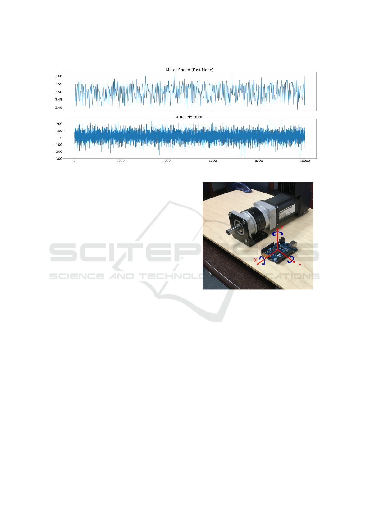
Figure 3: Examples of packet (top) and sensor (bottom) time series.

can turn it on or off, change or reverse its speed, etc.

The HMI sends a continual stream of commands. All

user input by way of the HMI is logged by the Rasp-

berry Pi and the command is passively forwarded to

the appropriate motor. The Arduino motion sensors

and network trafﬁc are continually collected by the

Raspberry Pi with timestamps in order to synchronize

all of the data with HMI user activity.

The sensor data is stored as Comma Separated

Values (CSVs) for X, Y, and Z rotation axes for both

the accelerometer and gyroscope. These axes rep-

resent the orientation of the attached sensors in the

three-dimensional space; this data is collected as a

constant stream as the sensor controller continuously

logs data from the motor at a ﬁxed sample rate of

10 thousand samples per second. The sensor data is

logged as ﬂoating point values that represent angular

velocity as degrees per second. We treat these motion

time series as potential side channels that leak net-

work information. The main data that could be leaked

includes the ModBus payload. Rather than being a

constant stream of data input, each payload arrives at

different times to the controller. To process the data

for time series clustering, the network data was pre-

processed, saving each data word of the payload in

the packet as separate time series. In each individ-

ual data payload there were 53 data words, leaving

53 potential time series that could have their infor-

mation leaked from the side channels. However, we

ﬁltered these time series further, removing payload

packets that did not change or were exactly periodic

(that is, always repeating). After ﬁltering, four data

words from the 53 time series remained that encoded

the speed setting of the motors (from the HMI) and

the actual speed measured by the motors. Each pair of

data words formed a 16-bit value for the speed setting

and the measured speed—thus these four time series

Figure 4: Orientations of sensors on Arduino relative to the

motor.

could be reduced to two time series that encoded the

speed into 16-bit values. We then used a Piecewise

Cubic Hermite Interpolating Polynomial (PCHIP) to

upsample the packet time series to match the dimen-

sions of the higher sample rate physical sensors. Fig-

ure 3 shows these time series examples for the mo-

tor speed packets and the acceleration data. Figure 5

shows heatmaps of all time series data, with all tri-

als concatenated. While the original setup also used

a man-in-the-middle (MITM) device to generate net-

work anomalies (Sinha et al., 2021), the portion of

the data set used in this paper was the baseline cal-

ibration data with no anomalies. Thus we are able

to use Granger time series clustering to investigate if

motion sensor data can be used as a side channel to

exﬁltrate network information. Speciﬁcally, this ex-

ﬁltrated network information was related to the en-

coding and measurement of motor speeds in Modbus

packets.

Side Channel Identiﬁcation using Granger Time Series Clustering with Applications to Control Systems

295

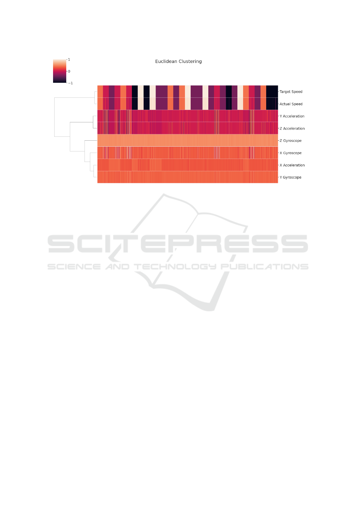
Figure 5: Euclidean hierarchical clustering of raw sensor and packet time series. Time series scaled to [-1, 1].

5 RESULTS

We applied our method to the data set described above

from (Sinha et al., 2021) to test it’s effectiveness as a

side channel identiﬁer. We also apply a traditional

clustering method for comparison.

5.1 Traditional Time Series Clustering

We ﬁrst clustered the time series using Euclidean dis-

tance as a baseline. This form of clustering only re-

ﬂects the similarity of the raw values in each time se-

ries. That is, the clusters represent time series which

have similar values at similar points in time. Figure

5 shows a normalized heatmap of each time series—

each row is one time series and colors reﬂect the value

of the time series. Moreover, we show a dendrogram

of the Euclidean cluster linkage on the left of the plot.

As we can see in Figure 5, the Target Speed and Ac-

tual Speed time series (from packet data) uniquely be-

long to their own cluster. This cluster is also dissim-

ilar to the sensor time series data. This indicates that

there is poor correlation between the packet data and

motion sensor data, from which we might infer that

these sensors do not contain any information about

the control packets and thus are poor side channels.

However, since feature-based clustering methods only

compare time series at a single point in time, they can

fail to pick up on relationships with a time lag or when

the features in each time series are dissimilar. Granger

causality, on the other hand, has the ability to account

for these kind of time series relationships, which al-

lows our Granger-based method to identify relation-

ships which traditional clustering methods do not, as

demonstrated in the next section.

5.2 Granger-based Clustering

Our data set was made up of individual trials in which

sensor and packet data were recorded while the mo-

tor was operating at different speeds. In order to cre-

ate the continuous time series needed for our method,

we randomly shufﬂed and concatenated these trials to

form one continuous time series per sensor. Perform-

ing a Dickey-Fuller (Dickey and Fuller, 1979) station-

arity test on all time series revealed that all time series

were stationary (p < 0.01 for all cases). This satis-

ﬁed the stationarity constraint of the Granger causal-

ity tests. These motion data time series served as our

group (potential side channels). The correspond-

ing packet data was also concatenated to form our X

group (data from the network that could potentially

be exﬁltrated). The X

time series contained six time

series (3 axes for acceleration and gyroscope) and the

time series contained two time series encoding the

speed, as discussed in Section 4.

To prevent any possible bias in our results from

ordering effects we performed our clustering on 10

independent shufﬂes of the data (i.e., different con-

catenations of the time series trials) and averaged the

results. With our X

and X

groups created, we per-

formed Granger clustering resulting in the Granger

maps,

G, displayed in Figure 6 and the clusters, A,

displayed in Figure 7. Figure 6 shows the two speed

related values along the horizontal axis and the mo-

ICISSP 2022 - 8th International Conference on Information Systems Security and Privacy

296

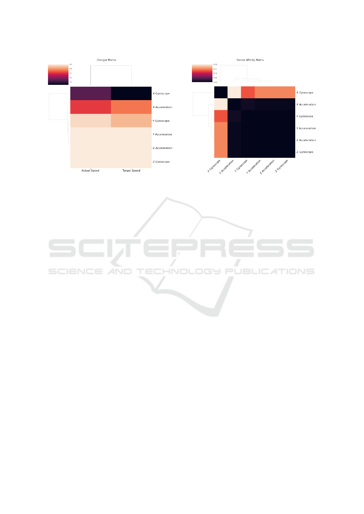
Figure 6: Clustermap of Granger matrix. Calculated as

mean of resulting granger matrices from 10 independent

shufﬂes of trials. Clustering is performed with γ = 10 and

t = 0.05 for ICS data.

tion sensor data along the vertical axis. The color of

the squares represent the strength of Granger causal-

ity found (after logistic transformation). Thus larger

values indicate a stronger relationship and therefore a

stronger potential for the sensor to be a side channel.

Outside the plot, a dendrogram is also shown and the

time series are ordered by their afﬁnity in the dendro-

gram. Figure 7 shows the pairwise cosine distances

that are calculated from each row of

G, thus reveal-

ing why the dendrogram linkages cluster. It is clear

from Figures 6 and 7 that there are two distinct clus-

ters, with the X gyroscope by itself in one cluster and

the rest of the sensors in the other. As we look fur-

ther down the dendrogram we see the X accelerom-

eter also begins to separate from the other sensors,

indicating that both sensors in the X direction have a

weaker Granger causal relationship with the control

packet data. This suggests that the X-axis gyroscope

is a poor side channel for the control system, whereas

signiﬁcant network information is potentially leaked

through physical signals in the Y and Z directions,

and to some degree from the X acceleration time se-

ries.

We can corroborate this conclusion by observing

the ICS system from (Sinha et al., 2021). If we look

at the orientation of the sensors in Figure 4, we can

see that the X direction is parallel to the axis of ro-

tation of the motor. Thus, the speed related vibra-

tions of the ICS would mainly occur in the Y and Z

directions, corroborating that the X-axis acceleration

is less powerful than Y or Z axes. Even so, Granger

clustering reveals that the X-axis acceleration data can

leak some information as it is strongly clustered with

Figure 7: Granger afﬁnity matrix. Calculated as pairwise

distances between rows of Granger matrix in Figure 6.

the other sensors. The gyroscope X direction, how-

ever, is a poor side channel. The speed of the motor

cannot be predicted by this time series as it is parallel

to the motion axis of the motor. This conclusion is in

stark contrast to Euclidean clustering, which revealed

that none of the sensor data were valid side channels.

It is important to note that the Granger cluster-

ing approach revealed these side channels without

any domain expertise regarding the ICS. Whether the

mechanism of data leakage was due to physical setup,

magnetic coupling with the sensors, or other means,

the analysis was able to reveal that packet informa-

tion was leaked by a subset of sensors. Moreover,

the analysis grouped the weaker response of the X-

acceleration with the other sensors, revealing that the

time series was potentially strong enough to be used

for exﬁltration. Beyond data leakage, the identiﬁed

side channels could also potentially be used to deﬁne

normal operation for the ICS. That is, Granger clus-

tering reveals that a set of time series are strongly re-

lated to the ICS network operation. If a MITM attack

were to occur, this relationship might be severed—for

instance if the actual motor speed was spoofed, the

causal sensor relationship would cease to exist. In this

way, such a side channel can be used to verify normal

operation of the ICS.

6 CONCLUSIONS

Granger clustering holds vast potential for ﬁnding

side channels in ICS. In this work we showed how

physical sensors can be related to control packet in-

formation using Granger-based clustering even when

Side Channel Identiﬁcation using Granger Time Series Clustering with Applications to Control Systems

297

a correlation-based method fails to ﬁnd these relation-

ships. Physical signals such as those used in this paper

as well as other non-functional information could be

evaluated with this method to determine if they pose a

risk as a side channel. Given the increase in complex-

ity of ICS and the ubiquity of physical sensors in ev-

eryday devices, identifying side channels like the ones

in this paper could signiﬁcantly inform design and se-

curity of ICS. Future work could include the use of a

non-parametric Granger causality test (Candelon and

Tokpavi, 2016) and the use of non-hierarchical clus-

tering methods for the Granger matrix.

REFERENCES

Anderson, R. (2020). Security Engineering, (Chap. 19 ‘Side

Channels’). John Wiley & Sons, Indianapolis, IN,

USA, 3rd edition.

Babu, B., Ijyas, T., Muneer P., and Varghese, J. (2017). Se-

curity issues in scada based industrial control systems.

In 2017 2nd International Conference on Anti-Cyber

Crimes (ICACC), pages 47–51.

Cai, L. and Chen, H. (2011). TouchLogger: inferring

keystrokes on touch screen from smartphone motion.

In Proceedings of the 6th USENIX conference on Hot

topics in security, HotSec’11, page 9, USA. USENIX

Association.

Candelon, B. and Tokpavi, S. (2016). A nonparametric test

for granger causality in distribution with application to

ﬁnancial contagion. Journal of Business & Economic

Statistics, 34(2):240–253.

Defays, D. (1977). An efﬁcient algorithm for a complete

link method. The Computer Journal, 20(4):364–366.

Dickey, D. A. and Fuller, W. A. (1979). Distribution of the

estimators for autoregressive time series with a unit

root. Journal of the American Statistical Association,

74(366a):427–431.

Dorf, R. and Bishop, R. (2017). Modern Control Systems.

Pearson Pub., Harlow, England, UK, 13th edition.

Genkin, D., Shamir, A., and Tromer, E. (2014). Rsa key

extraction via low-bandwidth acoustic cryptanalysis.

In Advances in Cryptology – CRYPTO14, pages 444 –

461. Springer Berlin Heidelberg.

Granger, C. W. (1969). Investigating causal relations

by econometric models and cross-spectral methods.

Econometrica: Journal of the Econometric Society,

pages 424–438.

Griswold-Steiner, I., LeFevre, Z., and Serwadda, A.

(2021). Smartphone speech privacy concerns from

side-channel attacks on facial biomechanics. Comput-

ers & Security, 100:102110.

Hojjati, A., Adhikari, A., Struckmann, K., Chou, E.,

Tho Nguyen, T. N., Madan, K., Winslett, M. S.,

Gunter, C. A., and King, W. P. (2016). Leave Your

Phone at the Door: Side Channels that Reveal Fac-

tory Floor Secrets. In Proceedings of the 2016 ACM

SIGSAC Conference on Computer and Communica-

tions Security, CCS ’16, pages 883–894, New York,

NY, USA. Association for Computing Machinery.

Ibing, A. (2012). On side channel cryptanalysis and sequen-

tial decoding.

Javed, A. R., Beg, M. O., Asim, M., Baker, T., and

Al-Bayatti, A. H. (2020). AlphaLogger: detecting

motion-based side-channel attack using smartphone

keystrokes. J Ambient Intell Human Comput.

Kocher, P., Horn, J., Fogh, A., , Genkin, D., Gruss, D., Haas,

W., Hamburg, M., Lipp, M., Mangard, S., Prescher,

T., Schwarz, M., and Yarom, Y. (2019). Spectre at-

tacks: Exploiting speculative execution. In 40th IEEE

Symposium on Security and Privacy (S&P’19).

Lipp, M., Schwarz, M., Gruss, D., Prescher, T., Haas, W.,

Fogh, A., Horn, J., Mangard, S., Kocher, P., Genkin,

D., Yarom, Y., and Hamburg, M. (2018). Meltdown:

Reading kernel memory from user space. In 27th

USENIX Security Symposium (USENIX Security 18).

McLaughlin, S., Konstantinou, C., Wang, X., Davi, L.,

Sadeghi, A., Maniatakos, M., and Karri, R. (2016).

The cybersecurity landscape in industrial control sys-

tems. Proceedings of the IEEE, 104(5):1039–1057.

Pliatsios, D., Sarigiannidis, P., Lagkas, T., and Sarigianni-

dis, A. G. (2020). A survey on scada systems: Secure

protocols, incidents, threats and tactics. IEEE Com-

munications Surveys Tutorials, 22(3):1942–1976.

Quisquater, J.-J. and Samdye, D. (2001). Electromagnetic

analysis (EMA): Measures and counter-measures for

smart cards. In Smart Card Programming and Secu-

rity (E-smart), pages 200 – 210.

Quisquater, J.-J. and Samdye, D. (2002). Side channel

cryptanalysis. In SEcurit

e des Communications sur

Internet – SECI02, pages 179 – 184.

Sinha, A., Taylor, M., Srirama, N., Manikas, T., Larson,

E. C., and Thornton, M. H. (2021). Industrial control

system anomaly detection using convolutional neural

network consensus. 2021 IEEE Conference on Con-

trol Technology and Applications (CCTA).

Stellios, I., Kotzanikolaou, P., Psarakis, M., Alcaraz, C.,

and Lopez, J. (2018). A survey of iot-enabled cyberat-

tacks: Assessing attack paths to critical infrastructures

and services. IEEE Communications Surveys Tutori-

als, 20(4):3453–3495.

ICISSP 2022 - 8th International Conference on Information Systems Security and Privacy

298