Searching for a Safe Shortest Path in a Warehouse
Aur
´
elien Mombelli, Alain Quilliot and Mourad Baiou
LIMOS, UCA, 1 Rue de la Chebarde, 63170 Aubi
`
ere, France
Keywords:
Shortest Path, Risk Aware, Time-dependant, A*, Reinforcement Learning.
Abstract:
In this paper, we deal with a fleet of autonomous vehicles which is required to perform internal logistics tasks
inside some protected areas. This fleet is supposed to be ruled by a hierarchical supervision architecture which,
at the top level, distributes and schedules Pick up and Delivery tasks, and, at the lowest level, ensures safety
at the crossroads and controls the trajectories. We focus here on the top level and deals with the problem
which consist in inserting an additional vehicle into the current fleet and routing it while introducing a time
dependent estimation of the risk induced by the traversal of any arc at a given time. We propose a model and
design a bi-level heuristic and an A*-like heuristic which both rely on a reinforcement learning scheme in
order to route and schedule this vehicles according to a well-fitted compromise between speed and risk.
1 INTRODUCTION
In an empty warehouse, an autonomous vehicle may
travel at full speed toward its destination. However, if
other autonomous vehicles are already working, trav-
elling inside the warehouse implies avoiding conges-
tion and costly accidents.
Monitoring a fleet involving autonomous vehicles
usually relies on hierarchical supervision. The trend
is to use three levels. At the low level, or embedded
level, robotic related problems are tackled for specific
autonomous vehicles like path following problems or
object retrieving procedures (Mart
´
ınez-Barber
´
a and
Herrero-P
´
erez, 2010). At the middle level, or local
level, local supervisors manage priorities among au-
tonomous vehicles and resolve conflicts in a restricted
area (Chen and Englund, 2016) who worked on cross-
road strategies. Then, at the top level, or global level,
global supervisors assign tasks to the fleet and com-
pute paths. This level must take lower levels into ac-
count in order to compute its own solution. For exam-
ple, (Wurman et al., 2008) compute the shortest path
thanks to the A* algorithm, but assign each task to the
fleet of autonomous vehicles using a multi-agent arti-
ficial intelligence in order to avoid conflict in arcs as
much as possible.
Redirecting autonomous vehicles to non-shortest
path may seem to increase the total travel time at first
but (Mo et al., 2005) showed that, in an airport, it ac-
tually decreased the total travel time and the conges-
tion time. With the same idea, several authors com-
puted the shortest path thanks to the A* algorithm,
first published by (Hart et al., 1968) in 1968. Then, if
any conflict is detected, an avoidance strategy is ap-
plied (Chen et al., 2013).
This study puts the focus on a global level: routing
and giving instructions to an autonomous vehicle in a
fleet. An autonomous vehicle, idle until now, is cho-
sen to carry out a new task. It must travel fast but it
must not take too many risks. Many articles propose
techniques to solve constrained shortest path prob-
lems, see (Lozano and Medaglia, 2013) for an exam-
ple. In 2020, (Ryan et al., 2020) used a weighted sum
of time and risks in Munster’s roads in Ireland to com-
pute a safe shortest path using an A* algorithm. In
their case, risk is a measure of dangerous steering or
braking events on roads. But these techniques mostly
cannot be applied here because the risk, in our case,
is time-dependent. One can search for the optimal
solution in a time-expanded network as did (Krumke
et al., 2014). A connection between two nodes in this
network represents the crossing of an arc in the static
network at a given time. Those kind of networks are
used, among other applications, for evacuation rout-
ing problems as did (Park et al., 2009).
This paper does not intend to study risks in a ware-
house. Therefore, we assume that we are provided
with a procedure which computes an expected value
of the risk of any arc at any time. This article aims
to answer the problem of finding a safe shortest path
while considering a warehouse structure, paths fol-
lowed by already working autonomous vehicles and a
risk estimation procedure. First, a precise description
of the problem is presented. Then, how to compute
Mombelli, A., Quilliot, A. and Baiou, M.
Searching for a Safe Shortest Path in a Warehouse.
DOI: 10.5220/0010780700003117
In Proceedings of the 11th International Conference on Operations Research and Enterprise Systems (ICORES 2022), pages 115-122
ISBN: 978-989-758-548-7; ISSN: 2184-4372
Copyright
c
 2022 by SCITEPRESS – Science and Technology Publications, Lda. All rights reserved
115

speed in a given path. Followed by two heuristics that
we designed to answer the problem. The paper ends
with numeric experiments and conclusions.
2 DETAILED PROBLEM
2.1 A Warehouse and the Risk Induced
by Current Activity
A warehouse is represented as a planar connected
graph G = (N,A) where the set of nodes N repre-
sents crossroads and the set of arcs A represents aisles.
For any arc a ∈ A, d
a
represent the minimal travel
time for an autonomous vehicle to go through aisle a.
Moreover, two aisles may be the same length but one
may stock fragile objects so that vehicles have to slow
down. This implies many different speeds among
aisles, thus many different minimal travel times.
Also, risk functions R
a
: t 7→ R
a
(t), generated from
activities of aisle a, are computed using the risk esti-
mation procedure we are provided with. Also, it is im-
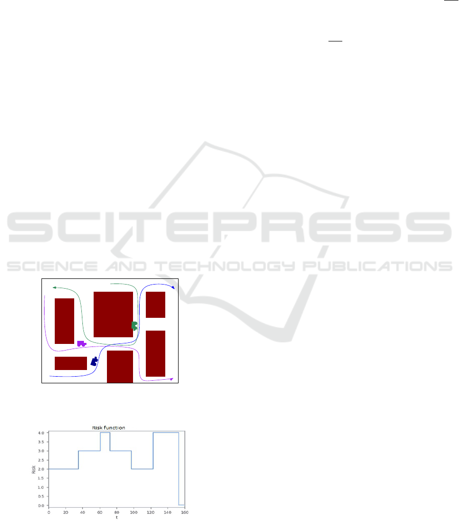
portant to note that the risk is not continuous. Indeed,
there is, in an aisle, a finite number of possible con-
figurations: empty, two vehicles in opposite direction,
etc. (see Figure 1). Each configuration is, then, asso-
ciated with an expected cost of repairs in the event
of accidents. Therefore, they are staircase functions
evaluated in a currency (euro, dollars, etc.). Figure 2
shows an example of a risk function of an aisle.
Figure 1: At time t, 3 aisles have 1 vehicle each. At the
next time , Blue and Purple join in the same aisle. One time
after, all 3 vehicles join, generating high risks in this aisle.
Figure 2: Risk function of an aisle.
From a risk function, we can estimate the risk an
autonomous vehicle takes in an aisle a between two
times t
1
and t
2
with v : t 7→ v(t) as its speed function
with Equation 1.
risk(t
1
,t
2
,v) = H(v)
Z
t
2
t
1
R
a
(t)dt (1)
We impose function H to be such that H(v) 
v
v
max
in order to model the fact that a decrease of the speed
implies a decrease of the risk. In further discussion,
H is set to H : v 7→

v
v
max

2
.
2.2 Our Problem: Searching for a Safe
Shortest Path Inside the Warehouse
An idle autonomous vehicle must now carry out a new
task inside the warehouse. Its task is to go from an
origin node o to a destination node p. We must de-
termine its path and its speed in each aisle of its path
while being provided with:
• The warehouse structure: G = (N,A) a planar
connected graph.
• The minimum travel time d
a
of every arc a.
• The estimated risk R
a
: t 7→ R
a
(t) of every arc a.
• The origin node o and the destination node p.
Then, we want to compute:
• Γ the path from o to p that will be followed by the
vehicle, along with entry time t
a
and leaving time
t
a+1
of every arc a of Γ.
If arc a is followed by arc b, t
a+1
= t
b
• v : t ∈ [t
a
;t
a+1
] 7→ v
a
(t) the speed to apply when
the vehicle is located inside every arc a of Γ.
Furthermore, a maximum risk value condition is
added. The warehouse manager will impose a maxi-
mum value of risk R
max
(quantified in currency, it can
correspond to the cost of replacing a vehicle in the
event of an accident) that an autonomous vehicle can
take for a task.
Finally, we want the program to be responsive and in-
teractive for managers of warehouses. Then, the ob-
jective is to determine quickly:
SSPP: Safe Shortest Path Problem
Compute path Γ together with entry times t
a
,
leaving times t
a+1
and speeds functions v
a
such that:
Global time: the arrival time in p is minimal.
Global risk:
∑
a∈Γ
risk (t
a
,t
a+1
,v
a
) ≤ R
max
ICORES 2022 - 11th International Conference on Operations Research and Enterprise Systems
116

As determining a whole speed function without
prior knowledge is complicated, we add a strong sim-
plification: We will only compute the average speed
in an arc. A consequence is that all speed functions
used will be constant. At lower decision levels, su-
pervisors will then have to choose real speed func-
tions respecting the average speed demanded (a con-
sequence is that travel time will be the same but risk
will decrease).
However this simplification creates anomalies: it may
happen that, in a specific aisle configuration, slowing
increases the risk taken instead of decreasing it.
For example, an autonomous vehicle wants to go
through an arc of minimal travel time 5 units. In this
arc, the estimated risk is null at its entry time for 5
units and is equal to 2 afterwards. Going at maximum
authorised speed will lead to a null risk but going at
half that speed will lead to a non-zero taken risk.
As determining the average speed is equivalent to
determining the exit time knowing the entry time, we
want to compute:
• Γ the path from o to p that will be followed by the
vehicle.
• t
i
the exit time of the i
th
arc of Γ.
With t
0
the entry time of the first arc of Γ and average
speed v
i
in the i
th
arc is fixed to v
i
=
d
i
t
i
−t
i−1
v
max
.
2.3 Why the Problem is Difficult in
Practice
To answer the problem with R
max
, a greedy heuristic
can be as follows:
• The chosen path is the shortest path (in terms of
minimal travel time)
• Every exit time is the first time such that the risk
taken r
i
in the i
th
arc verify Equation 2
i
∑
k=1
r
k
R
max
≤
i
∑
k=1
d
k
D
(2)
where D =
∑
a∈Γ
d
a
.
That way, every distance’s percentage travelled takes
less or exactly one risk’s percentage. It ensures the
risk will stay below R
max
at the end of the path.
However, let us take this example:
• the warehouse is made up of only 2 aisles of
length 5 and 5 respectively,
• there is a risk of 1 and 8 at all times on each aisle
respectively,
• both aisles must be traveled,
• R
max
is equal to 10.
The optimal solution goes at 0.5V
max
on the first
aisle (risk taken is 0.5
2
× (5/0.5) × 1 = 2.5), then
goes at
3
16
V
max
on the second aisle (risk taken is
(
3
16
)
2
× (5/
3
16
) × 8 = 7.5). The global travel time is
10 + 26.6 = 36.6 (rounded to the nearest 0.1) and the
risk is equal to R
max
.
The greedy solution goes at full speed on the first
aisle (risk taken is 1
2
× (5/1) × 1 = 5), then goes
at
1
8
V
max
on the second aisle (risk taken is (
1
8
)
2
×
(5/
1
8
) × 8 = 5). The global travel time is 5 + 40 = 45
and the risk is equal to R
max
.
There is a gap of almost 23% from the optimal
solution. And this gap widens each time the path gets
longer.
3 SOLVING THE SSPP WHEN
THE PATH IS FIXED
As the wanted output is made of two parts and the sec-
ond depends on the first, a sub-problem can be gener-
ated: if a path Γ, composed of n arcs, is chosen, what
is the optimal exit time of each arc that answers the
problem?
Let us denote by t
i
,i = 1 ... n the time when the vehi-
cle finishes the crossing of the i
th
arc of Γ. Then, Γ
being fixed, subproblem SSP(Γ) comes as follows:
SSP(Γ) Subproblem
Compute exit times t
1
,.. .,t
n
of Γ’s arcs
(and t
n
is the arrival time in p).
such that:
Global time: the exit time t
n
is minimal.
Global risk:
n−1
∑
i=0
risk (t
i
,t
i+1
,v
i
) ≤ R
max
A Dynamic Programming scheme simplifies a de-
cision by breaking it down into a sequence of decision
steps over time in a time space. As the exit time of the
i
th
arc depends on the exit of (i − 1)
th
arc, a Dynamic
Programming forward scheme is well fitted because
its time space is the set of nodes that we are visiting
one after another. The scheme we used is explained
in Figure 3.
With a very fine discretisation of the time, this Dy-
namic Programming scheme will find a good approx-
imation of the optimal solution. It will, however, take
a very long time. As we want the result quickly, we
will work on two aspects:
1. How to generate only a few decisions among the
best from a state?
2. How to compare two states and filter them to keep
a restricted number between nodes?
Searching for a Safe Shortest Path in a Warehouse
117

Time space I I = {0,... ,n}
The ordered set of nodes of the path.
Do not mistake time with the dynamic programming time space.
The latter will be called “nodes” from now on.
State space S s = (t,r) ∈ S
At node i, t (resp. r) is a feasible time (resp. risk) at node i.
Decision space δ ∈ DEC(i,s)
DEC(i,s) At node i, δ is a feasible exit time of the arc (i, i + 1).
It means that δ −t ≥ d
i+1
and r + risk (t,δ,v
i+1
) ≤ R
max
(where v
i+1
=
d
i+1
δ−t
v
max
).
Transition space (i,s)
δ
−→ (i + 1,s
0
)
Transition from (t,r) to (δ, r + risk (t, δ,v
i+1
))
Bellman Principle At node i + 1
Only non-dominated feasible states are kept: ∀(t
1
,r
1
),(t
2
,r
2
) ∈ S,
if t
1
≤ t
2
and r
1
≤ r
2
, (t
2
,r
2
) is dominated.
Search Strategy Scanning time I forwardly and construct the feasible State space accordingly.
Logical filtering The Greedy algorithm provides us with an upper bound of the optimal value.
Figure 3: Dynamic Programming scheme used.
Those questions lead to two different problems yet,
we will answer them both using a single function that
we call “state evaluation function”. In fact, if there
is a way to evaluate and sort a set of states, decisions
leading to those states can be sorted with the same or-
der. Then, decisions will be taken among the first ones
of the ordered set of decisions (see subsection 3.2 and
3.3). Afterwards, all generated states will be filtered
knowing their value (see subsection 3.4).
3.1 A State Evaluation Function
States are defined by the current time and risk taken to
travel to node i. The value of a state, given by a state
evaluation function, must be small for fast and safe
states (meaning states with small time and risk value)
and must be high for slow or risky states (meaning
states with high time or risk value). We propose a
function using a weighted sum: f
λ
: s = (t,r) 7→ r +λt
Where, λ represents the ratio between 1 time unit
and 1 risk unit. Of course, the ratio of the solution
is unknown. But searching for the optimal solution
contains searching for that ratio.
To approximate it, we propose to use a reinforce-
ment learning scheme applied to three values: λ
in f
,
λ
midst
and λ
sup
respectively a low, medium and high
estimation of λ
opt
. Therefore, at each node, after the
generation of new states, all λ values will be slightly
modified thanks to the previously generated states
(see subsection 3.5).
Another advantage of the reinforcement learned λ
values is that it can adapt itself in the middle of the
path: if a lot of too risky states are generated, λ values
will decrease to lower the value of slow states.
3.2 Generating Decisions Thanks to the
State Evaluation Function
Starting from state s = (t
i−1
,r
i−1
), a lot of new states
can be generated. But most of them are useless or
not promising enough to be considered (too slow, too
risky, slower and riskier than another state, etc.).
Thanks to the state evaluation function, we have a way
to evaluate quickly the state value of a decision for
a specific λ value (i.e. the value of the state if the
autonomous vehicle exits arc i at time t).
Because it is a function of one variable (t) and is in the
shape of a bowl (but sometimes not convex because of
the anomalies discussed at the end of subsection 2.2),
a dichotomy (using the left derivative) on the value of
t is used in order to find the global minimum of f
λ
.
This method gives the best decision possible for a
specific λ. But the value of λ
opt
is still unknown.
We propose to generate decisions by searching states
minimising f
λ
for a few λ values between the low and
high estimations of λ
opt
: λ
in f
and λ
sup
.
Those values will be distributed between λ
in f
and
λ
max
and led by λ
midst
(half of them uniformly dis-
tributed between λ
in f
and λ
midst
and half of them be-
tween λ
midst
and λ
sup
for example).
3.3 A Better Exploration of the Decision
Space
However, the decisions generated that way only take
the current arc into account. But it is not rare that the
optimal solution is faster and riskier in some arcs in
order to begin the next one before a high risk period.
Sometimes, given an optimal decision δ, it is not pos-
sible to associate δ with a λ parameter value such that
ICORES 2022 - 11th International Conference on Operations Research and Enterprise Systems
118

δ derive from the minimisation of function f
λ
.
In other words, decisions generated that way are
not enough to explore efficiently the decision space.
Therefore, other decisions must be generated that are
not a minimum of function f
λ
. However, the com-
puted minima can be used to lead those new decisions.
For example, the latter can be generated a few time
units before and after the former.
3.4 Filtering New States Knowing their
Value
Now that, from every state of node i − 1, new states
are generated, they are put together in an ordered set
(λ
midst
is used to order the set). Let us call this set S
i
.
The Bellman principle and the logical filter are first
applied: remove dominated states (states that are
slower and riskier than another one) and those which
finish after the computed upper bound. However, the
number of generated states is still exponential. To
keep a quick algorithm, the number of states in S
i
will
be bounded to S
max
.
If #S
i
> S
max
, which states must be removed? If
the λ
midst
value is very close to λ
opt
, the S
max
lowest
value states are kept and all others are removed from
S
i
. However, if it is not, a high state can be better than
the lowest state. Therefore, a method to determine
whether λ
midst
is a good approximation must be used.
We propose to compute the deviation of the state’s
risks of S
i
from travelled percentage of the path
(TravPer) as in Equation 3.
∆ =
∑
(t,r)∈S
i
(
r
R
max
− TravPer)
#S
i
(3)
If ∆’s absolute value is high, generated states take, on
average, too much risk or too little (meaning they can
go faster).
States are, then, removed depending on ∆’s value:
• If |∆| is “high” (close to 1), λ
midst
is supposed a
bad approximation:
j
#S
i
−S
max
3
k
states are removed from each third of
S
i
independently.
• If |∆| is “medium”:
j
#S
i
−S
max
2
k
states are removed
from the union of the 1st and 2nd third of S
i
and
the 3rd third of S
i
independently.
• If |∆| is “small” (close to 0), λ
midst
is supposed a
good approximation:
the first S
max
states are kept and all others are re-
moved.
3.5 Learning Lambdas Value
Because ∆ is the information about whether generated
states took, on average, too much, too little, or just
enough risk, it is also used to learn from the gener-
ated set. All lambdas are then moved according to the
sign and value of ∆, thanks to a descent algorithm, for
example. After experimenting, we chose the learning
equation to be Equation 4 because it gave us the best
results.
λ = λ × (1 − 0.2∆) (4)
More precisely, we need to compute the deviation ∆
of states generated by every λ independently. Because
we do not want to move a λ for “mistakes” of another
one. In other words, a λ value will be modified using
the deviation of the set of states generated by this λ
alone.
In the rest of the document, we used the above method
but below is another example of a learning process for
λ
in f
and λ
sup
.
Instead of considering the lambda values indepen-
dently, λ
in f
and λ
sup
can be seen as the bounds of an
interval and the learning process will be applied over
the width of this interval. Equation 4 will continue to
be applied on λ
midst
but another method must be used
to determine if the interval is wide enough. For exam-
ple, counting the number of states coming from λ
in f
(respectively λ
sup
) kept after the filtering process. If
there are a lot of them, λ
in f
(respectively λ
sup
) is too
close to λ
midst
. Then, a coefficient can be applied to
widen λ
midst
−λ
in f
(respectively λ
sup
−λ
midst
) (1.1 for
example).
Before this learning process, however, starting λ
values must be discussed.
If our algorithms have already been used in the ware-
house, their λ values will be kept as computed paths
can overlap and will then be already learned for the
next execution. However if it is not the case, several
other methods can be used to compute starting val-
ues.
We chose to apply preprocessing on the warehouse
by generating random paths solved by a greedy algo-
rithm that use Equation 4 to generate one exit time and
learn from all those decisions. The generation of ran-
dom paths can end after a fixed number of generations
or when the λ values seem to stabilise themselves.
4 SOLVING THE SSPP -
PROPOSED ALGORITHMS
Then, two algorithms can be created as follows:
• A decoupled method Algorithm 1: choose a path,
Searching for a Safe Shortest Path in a Warehouse
119

choose speed values on it, modify the path locally,
choose speed values again, keep the best, repeat.
• An A*-like method Algorithm 2: choose a node,
expand it by one arc, choose speed value on the
new arc, push the new arrival node with the other
unvisited nodes, repeat.
The A* algorithm is commonly used to search for the
shortest path in a very large graph because a lower
bound of expected value is associated with every un-
visited node. In so doing, the most promising nodes
will be visited first and all nodes having a greater
lower bound than an existing solution will not be used
at all. To solve the problem exactly, the A* algorithm
applied in the time expanded network of the ware-
house is enough but is very slow and does not fit our
requirements.
First, we introduce the decoupled heuristic to
solve the SSPP:
Algorithm 1: SSPP - Decoupled method.
Require: o and p, the origin and destination node.
Require: S
max
the maximum number of state to keep in the
Dynamic Programming scheme.
Require: Γ an initial path between o and p.
END = False
While not END Do
END = True
Generate V : neighborhood of Γ
For all neighbor ∈ V Do
Compute exit times of neighbor with the Dynamic Pro-
gramming scheme.
If neighbor finish earlier than Γ Then
Γ = neighbor
END = False
End If
End For
End While
Return Γ.
With no generation limit and no additional filter than
those of the Dynamic Programming scheme, this
heuristic can become an exact algorithm if the gener-
ated neighbourhood is large enough (modulo the time
units precision).
The generation method used is: for every couple of
nodes that are less or equal than two arcs away, pre-
compute a path between them, other than the shortest
one. The neighbour of a path is made by using the
pre-computed non-shortest path of a portion of that
path. The neighbourhood is then made of every pos-
sible neighbour of the path.
Finally, we introduce the heuristic based on A* al-
gorithm.
As the A* heuristic needs a function to estimate the
value of the remaining path, we propose the function:
b
λ
: x|(t,r,Γ) 7→ sp(x)

f
λ
(t,r)
length of Γ

.
This function uses the value of the current path to es-
timate the value of the shortest path from the current
node to the destination. A downside of this estimation
is if the start of the path is very risky, the function will
estimate the rest of the path to be very risky as well.
That way, the A* like heuristic will abandon this state
even if it is not true.
Algorithm 2: SSPP - A* like method.
Require: o and p, the origin and destination node.
Require: S
max
the maximum number of states to keep in
the Dynamic Programming scheme.
Let sp : x 7→ sp(x) be the length of the shortest path from x
to p.
Let b
λ
: x|(t,r,Γ) 7→ sp(x)

f
λ
(t,r)
length of Γ

be an estimation of
the remaining value to p.
Let Dict be a dictionary indexed by nodes of priority queues
which are ordered by f
λ
(x) + b
λ
(x) in ascending order.
push node = o|(t = 0,r = 0,Γ = []) in Dict.
At all times, Best
Dict
denotes the smallest value’s state
among heads of priority queues of Dict.
While node of Best
Dict
isn’t p Do
current = Best
Dict
= x
i−1
|(t
i−1
,r
i−1
,Γ
i−1
).
Pop Best
Dict
from corresponding priority queue.
Generate elongations (x
i
|t
i
,r
i
,Γ
i−1
+ [x
i−1
])
i
from current.
Push all elongations in their priority queues of D.
For all priority queue PQ ∈ Dict
If #PQ > S
max
Then
Filter PQ.
End If
End For
End While
Return Γ of Best
Dict
.
With no generation limit and no priority queue filter,
this heuristic becomes an exact algorithm (modulo the
time units precision).
Because this heuristic was too slow, another filter
was added: Each node is to be visited 2S
max
times
at most. However, short arcs are then privileged and
R
max
is reached before the end of the path.
Thankfully, a small change in the ordering of priority
queues was enough to compensate. Priority queues
are now separated in two halves: states {x|(t,r,Γ)}
that respect r < R
max
∗
t
t+sp(x)
first. Each ordered by
f
λ
(x) + b
λ
(x) in ascending order.
5 EXPERIMENTS
By those experiments, we want to compare the results
of the different algorithms presented before, along
with computation time. More precisely, a statistical
study of the parameters of proposed algorithms will
be presented first, then time and risk deviations from
the optimal solution will be compared.
We chose to implement all algorithms in Python3
ICORES 2022 - 11th International Conference on Operations Research and Enterprise Systems
120

Jupyter notebooks despite the speed requirement be-
cause we mostly want to compare the speed of the
different algorithms and because of its simplicity. All
notebooks have been launched from a Docker image
on an Intel Core i5-9500 CPU at 3GHz.
5.1 Creation of Random Instances
In Table 2, instance parameters are summarised:
Instances (“Name” column 1) are generated by creat-
ing a square grid n × n (“n” column 2) with random
minimum travel time (uniform distribution between 5
and 20). Because storage size may differ and aisles
may not form a perfect grid, a percentage of arcs are
dropped (“Drop” column 3). Then, on every arc, es-
timated risks are randomly generated (uniform dis-
tribution between 0 and 4) independently from each
other but arcs in the same instance are similarly active.
They are generated based on the average number of
configuration changes when passing through the aisle
at maximum speed (“Freq” column 4). Finally, we
choose the maximum risk accepted (“Max risk” col-
umn 5) as half of the risk taken if travelling at maxi-
mum authorised speed on the shortest path (length in
arcs, “SP len” column 6).
5.2 Statistical Study of Algorithms’
Parameters Value
Critical parameters will be studied below, but some
will not:
• The number of new states to generate from a pre-
vious one. As only the “best” states are generated,
it is not necessary to generate a lot a them. We set
this parameter to 5.
• The 3 discriminating values of ∆ to determine if
the value function is a “good” approximation or
not. As 0 ≤ |∆| ≤ 1, “small” values are below 0.2,
the “medium” value are between 0.2 and 0.5 and
the “high” values are above 0.5.
We will then study R
max
and S
max
values. To do so,
both algorithms will be used on 10 instances of ev-
ery group of parameters (100 instances in total). The
average objective values will be discussed below.
As a reminder, R
max
is the maximum risk accepted
and S
max
is the maximum number of states to keep
at each node of both algorithms. Temporarily, λ
in f
,
λ
midst
and λ
sup
are set to 0.2, 0.5 and 0.8. Both al-
gorithms along with the greedy one are used on 10
instances of every group presented above. The aver-
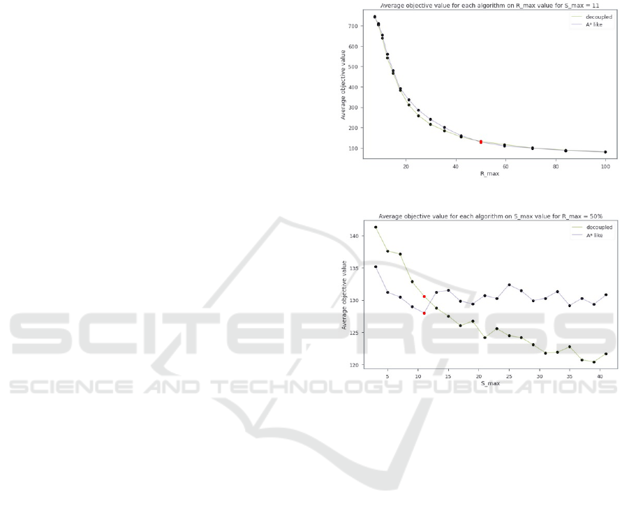
age objective values depending on R
max
for S
max
= 11
are presented in Figure 4.
Then, average objective values depending on S
max
for
R
max
= 50% of the risk taken at full speed on the
shortest path are presented Figure 5. Using those two
figures, we choose R
max
andS
max
such that both algo-
rithms compute nearly the same solutions. Hence, in
the rest of the paper, R
max
= 50% and S
max
= 11 will
be used.
Figure 4: Average objective values on R
max
for S
max
= 11.
Figure 5: Average objective values on S
max
for R
max
= 50%
of the risk taken on the shortest path at full speed.
5.3 Time and Risk Deviation From
Optimal
To compute the optimal solution we used a decoupled
strategy: for all paths from s to p, compute exit dates
with the Dynamic Programming scheme with no gen-
eration limit and no filter other than logical filters, al-
ways keeping the best. Optimal solutions and results
of proposed algorithms are presented in Table 1.
Rows named “Decoupled” show the results of the
decoupled heuristic.
Row “A*-like” shows results of the A*-like heuristic.
Row “Greedy” shows results of the greedy heuristic.
Row “Optimal” shows optimal solutions.
6 CONCLUSION
This Safe Shortest Path Problem in warehouses is a
very complex research subject and cannot be sum-
Searching for a Safe Shortest Path in a Warehouse
121

Table 1: Experimental results.
CPU time 01 02 03 04 05 06 07 08 09 10
Decoupled 0.03s 0.36s 0.67s 0.73s 4.56s 3.12s 0.06s 0.03s 0.70s 1.10s
A*-like 0.02s 0.21s 1.42s 0.17s 2.53s 3.68s 0.01s 0.03s 2.55s 0.98s
greedy 0.01s 0.01s 0.03s 0.02s 0.06s 0.06s 0.01s 0.01s 0.04s 0.04s
t
Optimal 38 83 165 63 189 220 31 41 165 118
Decoupled 39 97 169 65 190 241 32 52 172 128
A* like 39 97 177 66 196 264 33 54 186 121
greedy 103 108 190 69 223 267 35 54 208 134
risk
Optimal 10.98 79.75 68.27 72.12 176.98 215.83 33.90 23.20 91.54 90.11
Decoupled 10.50 78.24 67.30 57.62 176.75 216.48 34.27 26.26 91.72 94.79
A* like 10.50 80.01 68.35 58.07 176.50 216.15 34.08 21.02 90.50 94.15
greedy 11.50 74.80 68.60 56.50 177.80 216.80 32.80 26.00 91.20 94.30
Table 2: Instance parameters table.
Name n Drop Freq Max risk SP len
01 4 10 3 11.5 3
02 4 25 3 80.5 7
03 7 10 3 69.0 9
04 7 25 3 78.0 9
05 10 10 3 178.0 15
06 10 25 3 217.0 19
07 4 10 9 34.5 3
08 4 25 9 26.5 3
09 7 10 9 92.0 11
10 7 25 9 95.5 9
marised easily. In this paper, a very reductive hypoth-
esis has been taken: a path for an autonomous vehicle
is computed with average speeds only (i.e. consid-
ering entering and leaving aisles dates only). This
hypothesis leads us to create two heuristics: by de-
coupling path/phase resolution and resolving both at
the same time in an A* algorithm way. Experiments
show that the A*-like heuristic combined with rein-
forcement learning performs fairly behind the decou-
pled heuristic for some instances.
This study will be extended for several vehicles
and several tasks.
ACKNOWLEDGMENT
We want to acknowledge Susan Arbon Leahy, who
kindly accepted to proof read this article.
REFERENCES
Chen, L. and Englund, C. (2016). Cooperative Intersection
Management: A Survey. IEEE Transactions on Intel-
ligent Transportation Systems, 17(2):570–586.
Chen, T., Sun, Y., Dai, W., Tao, W., and Liu, S. (2013). On
the shortest and conflict-free path planning of multi-
agv systembased on dijkstra algorithm and the dy-
namic time-window method. 645:267–271.
Hart, P., Nilsson, N., and Raphael, B. (1968). A Formal Ba-
sis for the Heuristic Determination of Minimum Cost
Paths. IEEE Transactions on Systems Science and Cy-
bernetics, 4(2):100–107.
Krumke, S. O., Quilliot, A., Wagler, A. K., and Wegener,
J.-T. (2014). Relocation in carsharing systems using
flows in time-expanded networks. pages 87–98.
Lozano, L. and Medaglia, A. L. (2013). On an exact method
for the constrained shortest path problem. Computers
& Operations Research, 40(1):378–384.
Mart
´
ınez-Barber
´
a, H. and Herrero-P
´
erez, D. (2010). Au-
tonomous navigation of an automated guided vehicle
in industrial environments. Robotics and Computer-
Integrated Manufacturing, 26(4):296–311.
Mo, D., Cheung, K., Song, S., and Cheung, R. (2005).
Routing strategies in large-scale automatic storage
and retrieval systems. page 1.
Park, I., Jang, G. U., Park, S., and Lee, J. (2009). Time-
Dependent Optimal Routing in Micro-scale Emer-
gency Situation. pages 714–719.
Ryan, C., Murphy, F., and Mullins, M. (2020). Spatial risk
modelling of behavioural hotspots: Risk-aware path
planning for autonomous vehicles. Transportation Re-
search Part A: Policy and Practice, 134:152–163.
Wurman, P. R., D’Andrea, R., and Mountz, M. (2008). Co-
ordinating hundreds of cooperative, autonomous vehi-
cles in warehouses. 29:9–19.
ICORES 2022 - 11th International Conference on Operations Research and Enterprise Systems
122