AAEGAN Loss Optimizations Supporting Data Augmentation on

Cerebral Organoid Bright-ﬁeld Images

Clara Br

emond Martin

12 a

, Camille Simon Chane

1 b

, C

edric Clouchoux

2 c

and Aymeric Histace

1 d

ETIS Laboratory UMR 8051 (CY Cergy Paris Universit

e, ENSEA, CNRS), 6 Avenue du Ponceau, 95000 Cergy, France

Witsee, 33 Av. des Champs-

Elys

ees, 75008 Paris, France

Keywords:

Cerebral Organoid, Loss, Adversarial Autoencoder (AAE), Generation, Segmentation, t-SNE.

Abstract:

Cerebral Organoids (CO) are brain-like structures that are paving the way to promising alternatives to in vivo

models for brain structure analysis. Available microscopic image databases of CO cultures contain only a

few tens of images and are not widespread due to their recency. However, developing and comparing reliable

analysis methods, be they semi-automatic or learning-based, requires larger datasets with a trusted ground

truth. We extend a small database of bright-ﬁeld CO using an Adversarial Autoencoder(AAEGAN) after

comparing various Generative Adversarial Network (GAN) architectures. We test several loss variations,

by metric calculations, to overcome the generation of blurry images and to increase the similitude between

original and generated images. To observe how the optimization could enrich the input dataset in variability,

we perform a dimensional reduction by t-distributed Stochastic Neighbor Embedding (t-SNE). To highlight a

potential beneﬁt effect of one of these optimizations we implement a U-Net segmentation task with the newly

generated images compared to classical data augmentation strategies. The Perceptual wasserstein loss prove

to be an efﬁcient baseline for future investigations of bright-ﬁeld CO database augmentation in term of quality

and similitude. The segmentation is the best perform when training step include images from this generative

process. According to the t-SNE representation we have generated high quality images which enrich the

input dataset regardless of loss optimization. We are convinced each loss optimization could bring a different

information during the generative process that are still yet to be discovered.

1 INTRODUCTION

Cerebral organoids (CO) are brain-like structures that

are paving the way to promising alternatives to in

vivo models for brain structure analysis. Method im-

plementations such as automatic extraction of shape

parameters or size of organoid cultures, requires a

large amount of images (Kassis et al., 2019). The

scarcity of available data (worsened by the pandemic)

is currently a strong limitation to the development

of tools to support a more systematic use of CO

(Br

emond Martin et al., 2021). Data augmentation, a

prevalent method in the biomedical domain (Yi et al.,

2019), is a possible solution to overcome this issue.

Classical data augmentation strategies transform

the input images with a combination of rotations,

https://orcid.org/0000-0001-5472-9866

https://orcid.org/0000-0002-4833-6190

https://orcid.org/0000-0003-3343-6524

https://orcid.org/0000-0002-3029-4412

rescalings, etc, but the content variability that can be

observed when acquiring real bright-ﬁeld images is

not reproduced. Deep learning generative methods,

called Generative Adversarial Networks (GAN), can

solve this problem. Originally introduced by Good-

fellow et al, (Goodfellow et al., 2014), GANs are

constituted by a generator and a discriminator net-

work trained in an adversarial strategy. Since their

introduction GANs have evolved and variations such

as CGAN, DCGAN, InfoGAN, Adversarial Auto En-

coder (AAE) etc. have been proposed to increase the

size of biomedical datasets (Yi et al., 2019).

In this paper, we select and improve the best GAN

architecture (AAE) to generate cerebral organoid

bright-ﬁeld images. If the loss effect has already been

explored for others biological models in MRI (Lv

et al., 2021), to our knowledge, there is no systematic

comparative study proposed in the speciﬁc context of

CO bright-ﬁeld image generation that gives a quan-

titative appreciation of this effect. In particular, we

Brémond Martin, C., Simon Chane, C., Clouchoux, C. and Histace, A.

AAEGAN Loss Optimizations Supporting Data Augmentation on Cerebral Organoid Bright-ﬁeld Images.

DOI: 10.5220/0010780000003124

In Proceedings of the 17th International Joint Conference on Computer Vision, Imaging and Computer Graphics Theory and Applications (VISIGRAPP 2022) - Volume 4: VISAPP, pages

307-314

ISBN: 978-989-758-555-5; ISSN: 2184-4321

307

are interested in choosing a loss while guaranteeing

good quality of the generated data, as well as a good

variability of images obtained compared with the in-

puts in order to improve characterization tasks. The

contribution of this paper is to quantitatively investi-

gate the inﬂuence of various GAN-based approaches

and particularly AAEGAN losses in the speciﬁc case

of bright-ﬁeld CO image generation using quantita-

tive metrics from the literature and a dimensional re-

duction of parameters. The second contribution is to

compare data augmentation optimizations using a U-

Net-based segmentation task.

2 METHOD

2.1 Resources

Our dataset is composed of 40 images from an open

access database (Gomez-Giro et al., 2019). 20 patho-

logical and 20 healthy CO were numerized with a

bright-ﬁeld microscope over 3 days. The grayscale

images are 1088 × 1388 pixels. However, to compare

several networks within a reasonable time, the input

images are cropped and resized to 250 × 250 pixels,

maintaining the original proportions.

All algorithms are implemented in Python 3.6 (us-

ing an Anaconda framework containing Keras 2.3.1

and Tensorﬂow 2.1) and run on an Intel Core i7-

9850H CPU with 2.60 GHz and a NVIDIA Quadro

RTX 3000s GPU device.

2.2 Generative Adversarial Networks

Generative Adversarial Networks (GAN) are made

of two competing networks (Goodfellow et al.,

2014): the discriminative model (D) computes the

probability that a point in the space is an origi-

nal sample (o) from the dataset distribution(data).

However the generative model (G) maps the sam-

ples to the data space (z) by an objective func-

tion (F). D is trained to maximize the probability

of identifying the correct label (true/false) to both

generated (g) and original (o) samples. Simulta-

neously, G is trained to leverage the discrimina-

tor function expressed by: min

𝐺

max

𝐷

𝐹 (𝐷, 𝐺) =

𝐸

𝑜

𝑝

𝑑𝑎𝑡𝑎

[𝑙𝑜𝑔𝐷

𝑜

] + 𝐸

𝑔

𝑝

𝑔

[𝑙𝑜𝑔(1 − 𝐷(𝐺

𝑧

))].

Various GAN variations have been created since

its ﬁrst implementation. To ﬁnd the best suited net-

work, we consider ﬁve of the most known GAN-

architectures to increase the dataset: GAN (Good-

fellow et al., 2014) is the original implementation;

CGAN (Yi et al., 2019) gives to the generator in-

put the correct label (physiological or pathological);

Input

Generator

Encoder Decoder

Output

Discriminator

every 100 epochs

∆loss

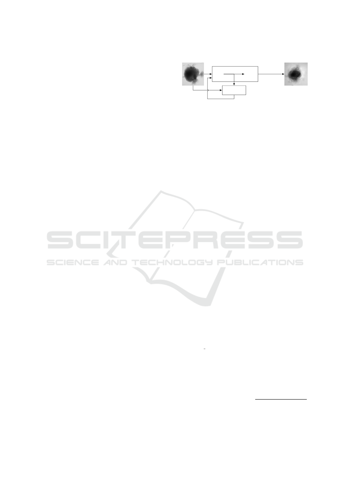
Figure 1: Experimental scheme of AAE supporting data

augmentation of cerebral organoids bright-ﬁeld images.

The generator tries to persuade the discriminator that it has

generated a true and slightly variable image of input dataset.

The discriminator tries to ﬁnd the true ones. They improve

each other by backpropagation, formulated by an objective

function based on a loss. Losses variations implemented

in this article are symbolized by Δ. Input image is from

(Gomez-Giro et al., 2019).

DCGAN (Yi et al., 2019) is constituted by a con-

volutional neural networks instead of the generator;

INFOGAN (Yi et al., 2019) uses the generated im-

ages at an epoch to train the subsequent; AAEGAN

(Makhzani et al., 2016) uses an autoencoder as a gen-

erator.

During a 1000 epoch duration training step, input

images of size 250 × 250 pixels are used to generate

synthetic images. In this work, the original 40 images

of the dataset are used to generate 40 synthetic im-

ages for a better follow-up by each architecture. The

number of images generated are chosen to guarantee

no mode collapse, as explained section 3.1.

2.3 Comparative Metrics

We calculate six metrics to compare the quality and

similitude of originals and generated images from the

various GAN architectures.

FID:Frechet Inception Distance satisﬁes most of the

requirements such as discriminability, or comparisons

of efﬁciency. This metric is used to determine the

image quality: a lower FID means smaller distance

between generated (g) and input data distribution (o

for original). In this equation, 𝜇 and Σ are respec-

tively the mean and co-variance of original and gen-

erated images: 𝐹𝐼𝐷(𝑜, 𝑔) = ∥𝜇

𝑜

− 𝜇

𝑔

∥

𝑇

(Σ

𝑜

+ Σ

𝑔

−

2(Σ

𝑜

𝑔

)

SSIM: The Structural Similarity Index compares pix-

els and their neighborhoods between two images us-

ing luminance, contrast and their structure. SSIM

has become a standard similarity measure to com-

pare synthetic and natural images even in the bi-

ological/medical domain. A high score stands for

high similitude: 𝑆𝑆𝐼 𝑀 (𝑜, 𝑔) =

(2𝜇

𝑜

𝜇

𝑔

+𝐶1) (2𝜎

𝑜

𝑔+𝐶2)

(𝜇

𝑜

+𝜇

𝑔

+𝐶1) ( 𝜎

𝑜

+𝜎

𝑔

+𝐶2)

Constants are added to stabilize the equations.

UQM:We have also implemented the universal qual-

ity metric which use the same contrast luminescence

VISAPP 2022 - 17th International Conference on Computer Vision Theory and Applications

308

and structures as the 𝑆𝑆𝐼 𝑀. A score of 1 indicate

an identical image. This metric is exposed below:

𝑈𝑄𝑀 (𝑜, 𝑔) =

4𝜇

𝑜

𝜇

𝑔

𝜇

𝑜

𝑔

(𝜇

𝑜

+𝜇

𝑔

) ( 𝜎

𝑜

+𝜎

𝑔

)

MI:In addition to these well established metrics, we

have also calculated the entropy-based Mutual Infor-

mation between input and generated images in order

to measure their correlation (highest score is equal to

1): 𝑀 𝐼 (𝑂, 𝐺) =

𝑜∈𝑂

𝑔∈𝐺

𝑃(𝑜,𝑔)𝑙𝑜𝑔

𝑃 (𝑜,𝑔)

𝑃 (𝑜) 𝑃 (𝑔)

Blur:To quantify the loss impact on the blurring

effect mentioned before, we use the blur met-

ric based on a sharpness quantiﬁcation of ob-

tained images and local variance value: 𝜎

𝑏 =

𝑚(𝑛−1)

𝑚

𝑖=1

𝑛−1

𝑗=1

[𝑝 (𝑖, 𝑗) − 𝑝

′

]

In this equation, 𝑚

and 𝑛 are subblocks of images, 𝑝(𝑜,𝑔) the predictive

residues of images vector and 𝑝

′

its mediane. The

lowest score of the global variance corresponds to the

sharpest images.

PSNR and MSE:To investigate the quality of gen-

erated images, we calculate the peak signal to noise

ratio and the mean square error: 𝑃𝑆𝑁 𝑅(𝑜, 𝑔) =

20log 10(𝑚𝑎𝑥(𝑜)) − 20 log 10(𝑀𝑆𝐸𝑜, 𝑔) and

𝑀𝑆𝐸 (𝑜,𝑔) =

𝑚𝑛

𝑚−1

𝑖=0

𝑛−1

𝑗=0

(𝑜(𝑚

𝑖

, 𝑛

𝑗

) − 𝑔(𝑚

𝑖

, 𝑛

𝑗

))

Here 𝑚𝑎𝑥(𝑜) corresponds to the maximum pixel

value of an original image (255).

We calculate 𝐹𝐼 𝐷 between each group of gener-

ated and the dataset of input images, whereas we com-

pute 𝐵𝑙𝑢𝑟 on each image and rendered as a mean. We

process 𝑆𝑆𝐼 𝑀, 𝑀 𝐼, 𝑃𝑆𝑁 𝑅, 𝑀𝑆𝐸, 𝑈𝑄𝑀 between

each input and generated images and their mean is

rendered for each group.

2.4 Loss Optimizations

To generate the most qualitative and similar images,

we choose to optimize the best architecture based

upon the previously described metrics. Whatever the

architecture considered, all the generated images are

somewhat blurry. We choose to overcome this phe-

nomenon by studying how the discriminator loss can

inﬂuence the quality of the image generation. We in-

troduce six loss with some of them known in litera-

ture to resolve similar issues (Kupyn et al., 2018; Lan

et al., 2020; Mao et al., 2017).

BCE: The most commonly used loss in GANs is the

binary cross entropy (BCE) calculated by (Makhzani

et al., 2016) with 𝑦 the real image tensor and 𝑦

′

the predicted ones: 𝐵𝐶𝐸 = −

𝑛

𝑖=1

(𝑦

𝑖

∗ (log(𝑦

′

𝑖

))) −

((1− 𝑦

𝑖

) ∗ (log(1− 𝑦

′

𝑖

))). The BCE loss is the baseline

of this work. Additionally, we have implemented ﬁve

discriminator losses which are chosen for their aim to

improve the generated images quality with respect to

contrast, sharpness, and blur effect.

BCE + L1: First, the original BCE is replaced with

BCE and a L1 normalisation (Wargnier-Dauchelle

et al., 2019). We hypothesize that such update could

improve the quality of the generation as reported in

image restoration tasks for instance: 𝐿1 =

𝑛

𝑖=1

|𝑜

𝑖

−

𝑔

𝑖

and 𝐵𝐶𝐸 𝐿1 = 𝐵𝐶𝐸 + 𝛼 ∗ 𝐿1 (10) 𝛼 is equal to

−

4, as in the original paper.

LS:In (Mao et al., 2017) the least square loss al-

lowed to avoid gradient vanishing in the learning pro-

cess step, contributing to create high quality images:

𝐿𝑆 =

𝑛

𝑖=1

(𝑜

𝑖

− 𝑔

𝑖

)

Poisson:In (Wargnier-Dauchelle et al., 2019), a Pois-

son loss is used to obtain more sensitive results

for segmentation tasks: 𝐿

𝑃𝑜𝑖𝑠𝑠𝑜𝑛

𝑛

𝑖=1

𝑔

𝑖

− 𝑜

𝑖

∗

log(𝑔

𝑖

+ 𝜖).

Wasserstein and Perceptual Wasserstein:The De-

blurGAN was developed to deblur images (Kupyn

et al., 2018), using a combination of the Wasserstein

and Perceptual loss. Since we are also interested in

deblurring the output images, we have tested both

losses with the proposed AAEGAN.

We launch loss optimizations on the best architec-

ture during 5000 epochs ﬁrst to train the model. Dur-

ing the training step, 250 × 250 pixel input images are

used to generate 40 synthetic images every 100 epoch.

The global representation explaining this training step

on the best architecture is shown Figure 1. We then

create a loss value per epoch representation, to high-

light when the training has to stop. We have stopped

the training at 2000 epochs which corresponds to the

plateau before the over-ﬁtting for each loss optimiza-

tion.

During the testing step based upon the model pre-

viously created, 40 images are created by each opti-

mization as explained in section 3.1. We then com-

pare the 40 images generated from each loss opti-

mization based upon the quality and similitude met-

rics described in section 2.3.

2.5 Dimensional Reduction

The dimensional reduction goal is to observe in the

same statistical space if, for each optimization, gener-

ated image representations are close or far from the

original image representations. We choose to per-

form a t-distributed Stochastic Neighboor Enbending

(t-SNE) dimensional reduction. Contrary to others

dimensional reduction methods, t-SNE preserves the

local dataset structure by minimizing the divergence

between the two distributions with respect to the loca-

tions of the points in the map. To avoid subjective or

calculated indexes, we perform t-SNE directly on fea-

tures of images extracted from the GAN networks. t-

SNE is constituted with Stochastic Neighbor Embed-

ding where ﬁrst an asymmetric probability (𝑝) based

AAEGAN Loss Optimizations Supporting Data Augmentation on Cerebral Organoid Bright-ﬁeld Images

309

on dissimilarities (symmetric) is calculated between

each object (𝑥

𝑖

), and its probably neighborhood (𝑥

𝑗

)

(Hinton and Roweis, 2003). The effective number of

local neighbors called perplexity (𝑘) is chosen man-

ually: 𝑝

𝑖, 𝑗

= exp



−

∥ 𝑥

𝑖

−𝑥

𝑗

∥

2𝜎

𝑖



𝑘≠𝑖

exp



−

∥ 𝑥

𝑖

−𝑥

𝑘

∥

2𝜎

𝑖



The larger the perplexity, the larger the variance

of a Gaussian kernel used to have an uniform in-

duced distribution. Thus we choose the maximal

value possible which is 80, the number of individ-

uals in our dataset. To match the original (𝑝

𝑖, 𝑗

)

and induced distributions (𝑝

′

𝑖, 𝑗

) in a low dimensional

space (the enbending aim), the objective is to mini-

mize the Kullback–Leibler (KL) cost function: 𝐶 =

𝑖

𝑗

𝑝

𝑖, 𝑗

log

𝑝

𝑖, 𝑗

𝑝

′

𝑖, 𝑗

. This minimization allows t-SNE

to preserve the dataset structure contrary to others di-

mensional reduction methods (as Principal Compo-

nent Analysis). Then a Student t-distribution with one

degree of freedom is used to avoid the crowding prob-

lem (van der Maaten and Hinton, 2008).

We use a momentum term to reduce the number of

iterations required (set at 1000 iterations at the begin-

ning) (van der Maaten and Hinton, 2008). The map

points have become organized at 450 iterations in a

scatterplot. Each point in the map corresponds to the

feature vector while the axes are the embedding fol-

lowing the similarity properties i.e. the neighborhood

of points. Each run of the t-SNE algorithm generates a

different setting of the scatterplot. The points location

might be different, but the grouping remains similar.

We have launched the t-SNE between original and all

the generated features 10 times to validate the similar

grouping. We have retrieved the best KL divergence

values between original and each generated distribu-

tions which could indicate a degree of similitude. A

low KL divergence means the two distributions are

close.

2.6 Segmentation

To determine the effect of data augmentation with the

AAE loss optimizations on a segmentation task, we

suggest to consider several training scenarios using a

U-Net architecture (Ronneberger et al., 2015). Seg-

mentation allows the extraction of an image content

from its background. Various segmentation proce-

dures exist but we have chosen U-Net for its advan-

tages to work well for small training sets with data

augmentation strategies, and to have already been

used for images of cleared CO (Albanese et al., 2020).

For comparison we perform 40 classical augmen-

tations involving ﬂip-ﬂops, rotations, whitenings, or

crops. Second, 40 images generated using an AAE

loss optimization are considered. The speciﬁc amount

of 40 is chosen in order to keep the balance between

original images and generated ones in the training

dataset, as explained further in section 3.1. To make

the performance evaluation more robust, a ”leave-

one-out” strategy is used, resulting in 40 training ses-

sions (numbers of images in our original dataset).

Thus each training is perform on 79 images. We

stopped the training at 1000 epochs with an average

time of training of more than 1 hour for each leave

one out loop (7 cases of augmentations × 40 images =

280 hours almost for the total training step). To com-

pare ground truth cerebral organoid content segmen-

tation (gt) and U-Net (u) ones in various conditions,

mean DICE scores are calculated as : DICE(𝑔𝑡,𝑢) =

2|𝑔𝑡∩𝑢|

|𝑔𝑡 |+|𝑢|

To highlight real/false positive/negative segmenta-

tion we created a superimposed image composed by

the ground truth and a sample of each segmentation

resulting from the various trainings. We updated the

pixels values in magenta (255, 0, 255) the false posi-

tive cerebral organoid segmentations and, in cyan (0,

255, 255) the false negatives.

3 RESULTS

We aim at generating qualitative images of cerebral

organoid by GAN strategies to increase the open-

source dataset (Gomez-Giro et al., 2019).

To determine the maximum number of images

generated without collapse, we calculate the SSIM

between original and generated images. We set that

the maximal similitude without creating a twin con-

tent is 0.90 (the maximum of similitude between two

original images is only of 0.87). Generated images

are at the minimum 45 % similar to original images.

When we double the generative process, some identi-

cal images appear. Thus we choose to generate only

40 images for each case in the testing phase to avoid

these duplicates.

3.1 GAN Architecture Choice

To verify the best suited GAN architecture for cere-

bral organoid bright ﬁeld images, we ﬁrst compare the

original images and the ones generated using the ﬁve

architectures.

In Table 1, sample images produced with GAN,

CGAN and AAEGAN are the most resembling im-

ages compared to the originals. Mode collapse is the

most seen in GAN and CGAN architectures as re-

ported in the literature. We can observe also a strong

noise for these two architectures results with a white

imprint around the shape of the organoid in the GAN

VISAPP 2022 - 17th International Conference on Computer Vision Theory and Applications

310

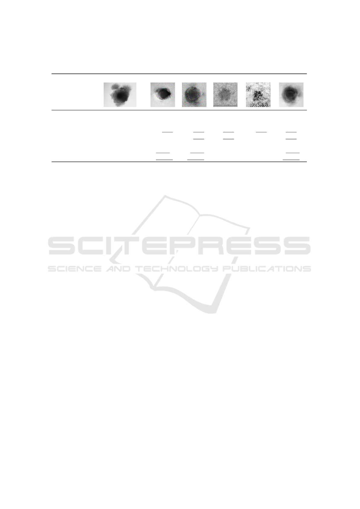
Table 1: Image quality and similitude of cerebral organoids generated by various GAN architectures. Scores within the

original range are underlined, best values are displayed in bold.

Original GAN CGAN DCGAN INFOGAN AAE

metric best

FID low 0.47 ≤ 𝑥 ≤ 0.80 2.02 2.13 ≥ 4 2.89 1.20

SSIM high 0.65 ≤ 𝑥 ≤ 0.71 0.12 0.12 0.27 0.10 0.63

UQM high 0.63 ≤ 𝑥 ≤ 0.87 0.79 0.80 0.69 0.66 0.81

MI high 0.21 ≤ 𝑥 ≤ 0.47 0.17 0.24 0.25 0.19 0.37

BLUR low 0.10 ≤ 𝑥 ≤ 86.28 2504.24 7561.47 704.48 724.38 135.93

PSNR low 11.90 ≤ 𝑥 ≤ 16.60 12.16 12.64 28.35 28.35 12.89

MSE low 93.25 ≤ 𝑥 ≤ 106.23 105.41 103.07 107.12 107.14 102.72

case. While AAEGAN generated images are char-

acterized with blurry contours, DCGAN and INFO-

GAN generate a divergent background making the

images difﬁcult to exploit. To verify these observa-

tions, we calculate qualitative and similitude metrics,

introduced in the section 2.3, by pairing ﬁrst original

images and then original and generated images.

Table 1, presents these results. For the output im-

ages, we underline the metric values within range of

the original images. We observe only a low propor-

tion of architecture metric within the original range.

Indeed, only the AAEGAN and the CGAN answer

to only four metrics (UQM, MI, PSNR, MSE) on

the seven calculated and only the UQM is within the

range of original ones for all the architectures. Re-

garding FID, SSIM, UQM, and MI scores, AAEGAN

generate the most comparable images to the original

ones.

In term of quality, this architecture generate the

sharpest images, even if the blur index is higher than

original images indexes. All the architectures express

MSE of between the minimal and maximal values of

this metric calculated for the original images. How-

ever, regarding the PSNR only the GAN, CGAN and

AAEGAN produce images with a score of between

the original images limits. To summarize, according

to the metric values, AAEGAN is the most suited ar-

chitecture to generate cerebral organoid images.

3.2 AAEGAN Loss Optimization

Once we have conﬁrmed AAEGAN is the most suited

generation architecture for our study, we update the

discriminative loss of AAEGAN in order to evaluate

the corresponding inﬂuence on the generated images

quality. Results are shown in Table 2, using the same

metrics for quality (PSNR, MSE and Blur) and simil-

itude (FID, UQM, SSIM and MI) of images.

Table 2 shows one of the 40 images generated for

each of the six AAE variations. While some of the

generated samples are blurry and present a white im-

print (BCE, BCE+L1, LS), others show sharper edges

and less visible imprints (Poisson, Wasserstein and

Perceptual Wasserstein). For this group of losses,

only a few of the generated data seem to be identi-

cal to the input images: these networks do not suffer

from mode collapse.

To quantitatively conﬁrm the visual analysis of the

generated images, we calculate comparative metrics

between original and generated datasets. Results are

shown Table 2. The AAEGAN loss optimizations al-

low generated images to be within the range on ﬁve

metrics with the Wasserstein and Perceptual Wasser-

stein loss (against four for the other loss). Indeed, the

Blur index is with these two optimizations within the

range of original images. Of the 7 metrics calculated,

only FID and SSIM are not in the range for all the

optimizations. However, the FID for the Perceptual

Wasserstein loss is quite close to the upper bound of

the input range (0.82 vs. 0.80).

Quantitatively, Wasserstein and Perceptual

Wasserstein networks generate better image quality

than other networks, based on lower PSNR, MSE

score and Blur index. However they are still higher

than the original scores shown in Table 1.

Otherwise, the similarity seems to depend on the

architecture. Based upon the FID, the Perceptual

Wasserstein loss generates the most similar images.

MI is higher for the images generated using Wasser-

stein networks. However, compared to images pro-

duced with BCE and Poisson, images produced with

Perceptual Wasserstein loss are not similar to the orig-

inal dataset regarding the SSIM. Images generated

with a Poisson or LS loss have the best UQM index.

The Perceptual Wasserstein loss is the most ap-

propriate loss optimization for generating cerebral

organoid images with the AAEGAN. It performs best

AAEGAN Loss Optimizations Supporting Data Augmentation on Cerebral Organoid Bright-ﬁeld Images

311

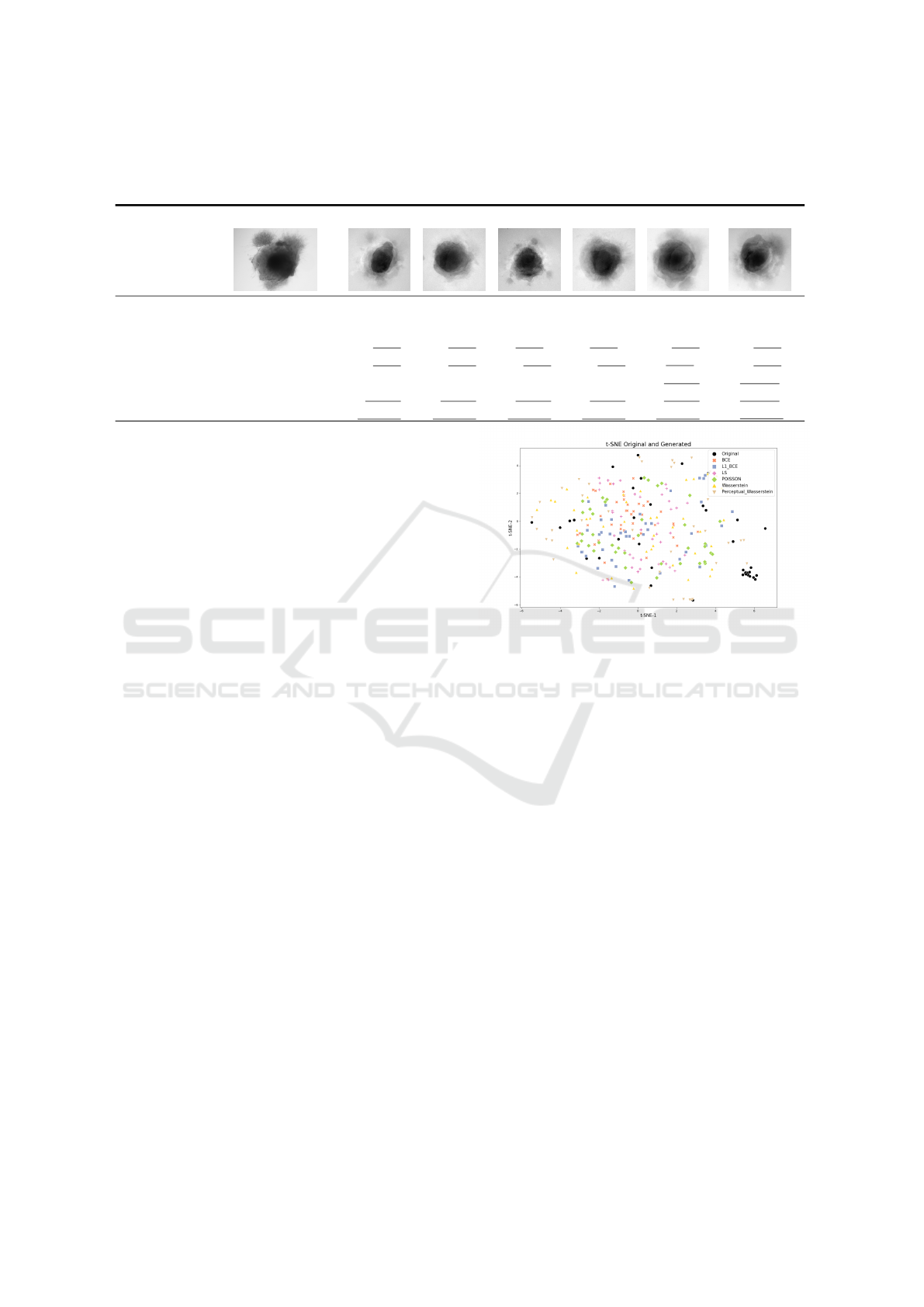
Table 2: Sample of images generated for each AAE loss variation. We have calculated metrics on generated images from

each AAE loss variations, with the BCE loss as the baseline. Scores within the original range are underlined, best values are

displayed in bold.

Original BCE BCE + L1 LS Poisson Wass. Per. + Wass.

metric best

FID low 0.47 ≤ 𝑥 ≤ 0.80 1.20 1.41 1.33 1.41 1.10 0.82

SSIM high 0.65 ≤ 𝑥 ≤ 0.71 0.63 0.62 0.60 0.63 0.62 0.50

UQM high 0.63 ≤ 𝑥 ≤ 0.87 0.83 0.83 0,84 0,84 0.83 0.82

MI high 0.21 ≤ 𝑥 ≤ 0.47 0.37 0.39 0.36 0.41 0.46 0.42

BLUR low 0.10 ≤ 𝑥 ≤ 86.28 135.93 116.30 135.01 106.71 59.84 59.00

PSNR low 11.90 ≤ 𝑥 ≤ 16.60 13.47 13.74 13.53 13.74 13.17 12.86

MSE low 93.25 ≤ 𝑥 ≤ 106.23 103.13 103.35 104.01 103.33 103.11 102.93

for four metrics and is within the original range for

ﬁve metrics.

3.3 Dimensional Reduction

To analyze all at once the similitude and the vari-

ability of the generated images with AAEGAN loss

optimization, we study images in the same statistical

space. We implement a dimensional reduction on the

features extracted on images in the generative process

with t-SNE, see Figure 2. The ﬁrst observation that

can be made is the maintenance of similar positions in

the map between original and generated images and

that whatever the loss optimization. Some original

images constitute a cluster and are almost foreigner

to the generated ones. This could be explained by the

incapacity of generated images to replicate a back-

ground similar to the bright-ﬁeld acquisition with a

light gradient. While at the exterior of the map im-

ages generated with a Poisson a Wasserstein or a Per-

ceptual Wasserstein loss are represented, inside the

map BCE, BCE+L1, and LS losses are. This observa-

tion suggests that each loss optimization could bring

different information during the generative process.

We compare the KL divergences between original and

generated images which remains similar (all results

are approximating the null : inferior at 0.3). To sum-

marize, loss optimizations generate similar contents

to original images keeping its variability and creating

intermediate shapes not seen in original population.

3.4 Segmentation

To illustrate the inﬂuence of generated images by an

optimised AAEGAN against classical data augmen-

tation, we suggest to tackle a segmentation task in a

leave-one-out strategy (n=79 for training and n=1 for

testing). We choose the classic U-Net architecture and

Figure 2: t-SNE representation of original and generated

images with optimized AAEGAN.

we consider the different losses to compare the seg-

mentation performance for each data augmentation.

Psychovisually, samples in Table 3 are the best

segmented with a training involving images result-

ing from the AAEGAN Perceptual Wasserstein opti-

mization. They show the less false positive and nega-

tive segmentations compared to others AAEGAN op-

timizations and to classical data augmentation. Quan-

titatively the mean DICE index highlight the segmen-

tation performance. Results are summarized in Table

3. Mean DICE index is higher for segmented images

with Perceptual Wasserstein augmentation, in accor-

dance with the selected visual illustration.

In conclusion, images generated from Perceptual

Wasserstein AAEGAN allow a more accurate seg-

mentation than other AAEGAN loss, in accordance

with previous results on quality. The inﬂuence of the

Perceptual loss combined with Wasserstein distance,

such as a data attachment term based on the difference

of generated and images features maps, improve their

sharpness and textural information, making it a viable

strategy for data augmentation in this context.

VISAPP 2022 - 17th International Conference on Computer Vision Theory and Applications

312

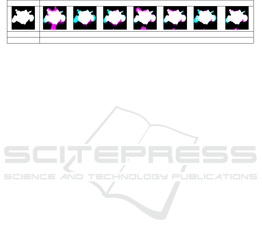
Table 3: Sample Cerebral Organoid image (left) with ground truth (GT) segmentation (our baseline), compared to Classical

and AAEGAN-based data augmentation, and the corresponding Mean DICE index and Standard Deviation (SD). Pixels are

colored according to the following legend: Black and white represent respectively true negatives and true positives while

magenta highligths false positives and cyan a false negatives. The best Dice index is displayed in bold.

GT Classic BCE BCE + L1 LS Poisson Wass. Per. + Wass.

Mean DICE 0.87 0.85 0.87 0.86 0.87 0.88 0.90

SD 0.03 0.05 0.05 0.14 0.09 0.05 0.04

4 DISCUSSION

This paper presents for the ﬁrst time to our knowledge

data augmentation of cerebral organoids bright-ﬁeld

images, using an Adversarial Autoencoder with var-

ious loss optimizations. The Perceptual Wasserstein

discriminator loss optimization outperforms the state-

of-the-art original article to generate these images, ac-

cording to the metrics used. Nevertheless, our dimen-

sional reduction experiments suggest all the loss op-

timizations could bring some variability to the gen-

erative process while remaining similar to the origi-

nal dataset. Approaching a segmentation experiment,

images generated with a Perceptual Wasserstein loss

could bring a better precision to a segmentation task.

Other losses may be interesting for different tasks.

Synthetic images generated with AAEGAN are

coherent with original dataset quality contrary to

other architectures, with almost no collapse mode but

also adding a sought diversity similar to the acquisi-

tion of the original dataset. An update of this archi-

tecture (for example replacing the autoencoder part by

a U-Net) may improve these results. Results remains

exploratory with the mentioned small dataset we used.

Improvements could be augmenting the number of in-

put images for all of the architectures, increasing the

training time for DCGAN and, giving to the INFO-

GAN generator only high-quality images to avoid the

divergence behavior. We only optimize the best archi-

tecture for time consideration, but the effect of loss

variations on others architectures may be interesting

to quantify.

The Perceptual Wasserstein loss optimization of

AAEGAN performs best according to metrics. Other

loss optimizations show also high similitude, though

with a lower quality. However, the dimensional re-

duction experiment suggests that several loss could

be used to generate more images and a good diver-

sity enriching the original training set. In this context,

we plan to explore what type of information each loss

brings during the image generation. We aim at trying

others embedded losses (already used for segmenta-

tion tasks) during the generative process based upon

high level prior like object shape, size topology or

inter-regions constraints (El Jurdi et al., 2021). These

losses could be used on condition that the morpholog-

ical development of CO is better characterized.

Attempting to distinguish the contribution of each

loss optimization, this strategy can potentially bring

better pixel-wise precision for segmentation tasks.

Shown here as a proof of concept, using a U-Net

architecture, we demonstrate the Perceptual Wasser-

stein loss can fruitfully enrich the original dataset.

This may also show a kind of regularization achieved

by the Perceptual loss leading to a good variability of

generated data without being too generic. The contri-

bution of others loss could not been highlighted in this

task. Nevertheless, segmentation could be even more

appropriate with algorithms suited for small datasets

or increasing the training step.

We plan also to train the segmentation task with

all the generated images (whatever the optimization)

in order to observe the modulation of its accuracy. In-

deed, we plan to extract morphological parameters,

such as areas, perimeters or higher-order statistics

needed for the growth follow-up of cerebral organoid

cultures on segmented images. In this work, we only

segmented organoid vs. non organoid regions. We

aim at reproducing the same work differentiating the

peripheral and the core zones of the cerebral organoid

in these images.

There is still room for improvement in the pro-

posed AAEGAN network strategy. First, to propose

a quantitative evaluation of the generalization of the

results obtained on cerebral organoid bright-ﬁeld im-

ages : we would like to use this methodology on oth-

ers bright-ﬁeld biomedical images. Biological experts

aim at psychovisually evaluating the generated im-

ages, and strengthen the quantitative evaluation pro-

posed. In particular, we project to validate the suit-

ability of the metrics we use and observe the training

effect on the segmentation task with only validated

images by biological experts.

AAEGAN Loss Optimizations Supporting Data Augmentation on Cerebral Organoid Bright-ﬁeld Images

313

Second, we chose to focus only on the use of an

AAEGAN architecture to generate our images, we

aim at comparing these results with other types of

GANs such as CycleGAN or PixtoPix using U-Net

in its generator (Yi et al., 2019). Then, we have to

mention the resembling of original images in the t-

SNE right corner. It appears generated images could

not really generate a similar background such as the

lightning gradient of some bright-ﬁeld acquisition in

white light. To resolve this issue, we aim at studying

the effect of a similar bright-ﬁeld background injec-

tion during the generative process.

Finally, given the input dataset containing phys-

iological and pathological models of CO, it would

be interesting to investigate the generation of speciﬁc

pathological content in future studies.

5 CONCLUSION

This study answer to the ﬁrst emerging issue in the

cerebral organoid ﬁeld highlighted in (Br

emond Mar-

tin et al., 2021) i.e the lack of datasets. These

ﬁrst results show that small databases augmentation

of cerebral organoids bright-ﬁeld images is possi-

ble using GANs. Particularly the AAEGAN Per-

ceptual Wasserstein loss optimisation generates the

most qualitative content, remains similar to the orig-

inal dataset and images it generates are useful to im-

prove a segmentation task. However it remains to

discover what kind of information other loss opti-

mizations with coherent diversity to the initial dataset

could bring during the generative process. This data

generation strategy will be valuable to develop char-

acterization methods on CO by enabling large statisti-

cal study, but also to develop deep-based approaches

for classiﬁcation and characterization of the various

morphologies. Such characterization could help to

better understand the growing process once in ade-

quate cultures and help to use cerebral organoids as

models for neuropathological disease or for testing

therapeutics.

REFERENCES

Albanese, A., Swaney, J. M., Yun, D. H., Evans, N. B.,

Antonucci, J. M., Velasco, S., Sohn, C. H., Arlotta,

P., Gehrke, L., and Chung, K. (2020). Multiscale 3D

phenotyping of human cerebral organoids. Scientiﬁc

Reports, 10(1):21487.

emond Martin, C., Simon Chane, C., Clouchoux, C., and

Histace, A. (2021). Recent Trends and Perspectives in

Cerebral Organoids Imaging and Analysis. Frontiers

in Neuroscience, 15:629067.

El Jurdi, R., Petitjean, C., Honeine, P., Cheplygina, V.,

and Abdallah, F. (2021). High-level prior-based loss

functions for medical image segmentation: A sur-

vey. Computer Vision and Image Understanding,

210:103248.

Gomez-Giro, G., Arias-Fuenzalida, J., Jarazo, J.,

Zeuschner, D., Ali, M., Possemis, N., Bolognin,

S., Halder, R., J

ager, C., Kuper, W. F. E., van Hasselt,

P. M., Zaehres, H., del Sol, A., van der Putten,

H., Sch

oler, H. R., and Schwamborn, J. C. (2019).

Synapse alterations precede neuronal damage and

storage pathology in a human cerebral organoid

model of CLN3-juvenile neuronal ceroid lipofus-

cinosis. Acta Neuropathologica Communications,

7(1).

Goodfellow, I. J., Pouget-Abadie, J., Mirza, M., Xu, B.,

Warde-Farley, D., Ozair, S., Courville, A., and Ben-

gio, Y. (2014). Generative Adversarial Networks. In

Proceedings of NIPS, page 2672–2680.

Hinton, G. and Roweis, S. (2003). Stochastic neighbor em-

bedding. Advances in neural information processing

systems, 0(no):857–864.

Kassis, T., Hernandez-Gordillo, V., Langer, R., and Grifﬁth,

L. G. (2019). OrgaQuant: Human Intestinal Organoid

Localization and Quantiﬁcation Using Deep Convolu-

tional Neural Networks. Scientiﬁc Reports, 9(1).

Kupyn, O., Budzan, V., Mykhailych, M., Mishkin, D., and

Matas, J. (2018). DeblurGAN: Blind Motion Deblur-

ring Using Conditional Adversarial Networks. Pro-

ceedings of the IEEE Conference on Computer Vision

and Pattern Recognition, pages 8183–8192.

Lan, L., You, L., Zhang, Z., Fan, Z., Zhao, W., Zeng, N.,

Chen, Y., and Zhou, X. (2020). Generative Adversar-

ial Networks and Its Applications in Biomedical In-

formatics. Frontiers in Public Health, 8.

Lv, J., Zhu, J., and Yang, G. (2021). Which GAN? A

comparative study of generative adversarial network-

based fast MRI reconstruction. Philosophical Trans-

actions of the Royal Society A: Mathematical, Physi-

cal and Engineering Sciences, 379(2200):20200203.

Makhzani, A., Shlens, J., Jaitly, N., Goodfellow, I., and

Frey, B. (2016). Adversarial Autoencoders. Interna-

tional Conference on Learning Representations.

Mao, X., Li, Q., Xie, H., Lau, R. Y. K., Wang, Z., and Smol-

ley, S. P. (2017). Least Squares Generative Adver-

sarial Networks. IEEE International Conference on

Computer Vision (ICCV), pages 2813–2821.

Ronneberger, O., Fischer, P., and Brox, T. (2015). U-

Net: Convolutional Networks for Biomedical Im-

age Segmentation. arXiv:1505.04597 [cs]. arXiv:

1505.04597.

van der Maaten, L. and Hinton, G. (2008). Visualizing data

using tsne. Journal of Machine Learning Research,

9(1):2579–2605.

Wargnier-Dauchelle, V., Simon-Chane, C., and Histace, A.

(2019). Retinal Blood Vessels Segmentation: Im-

proving State-of-the-Art Deep Methods. In Computer

Analysis of Images and Patterns, volume 1089, pages

5–16. -, Cham.

Yi, X., Walia, E., and Babyn, P. (2019). Generative Adver-

sarial Network in Medical Imaging: A Review. Medi-

cal Image Analysis, 58:101552.

VISAPP 2022 - 17th International Conference on Computer Vision Theory and Applications

314