
Study of Three WFS for the Modular System in a Portable AO
Instrument: ALIOLI
Esther Soria
1,2 a
and Roberto L
´
opez
1,2 b
1
Instituto de Astrof
´
ısica de Canarias, C/V
´
ıa L
´
actea s/n, La Laguna, E-38205, Spain
2
Departamento de Astrof
´
ısica, Universidad de La Laguna, La Laguna, E-38200, Spain
Keywords:
Adaptive Optics, High Resolution, Wavefront Sensor, Wavefront Corrector, Medium Sized Telescopes.
Abstract:
Adaptive optics (AO) systems correct atmospheric turbulence in real time and they are normally designed for
large telescopes but not for modest due to their cost. In this paper, we propose a portable AO instrument,
named ALIOLI, capable of be installed in different medium and small-sized telescopes. The novelty of this
new instrument is the modularization of its components which allows great flexibility in the design, being
possible easily adapt the instrument to the working telescope or observing technique by adjusting each module
independently. Here we present the instrument concept and a preliminary design for its installation in the
Carlos Sanchez Telescope ( 1.5m, Teide Observatory (Canary Islands)). The Wavefront Sensor (WFS)
module is intended to be used with three different WS, Shack-Hartmann, Two Pupil Plane Position and non-
modulated Pyramidal, allowing a joint configuration for comparative studies. A comparison of the response of
these sensors has been carried out by simulating the instrument in Python. The simulation results demonstrate
the goodness of the applied algorithms and the higher linearity and precision of the SH WFS in comparison
with the others two.
1 INTRODUCTION
The wavefront (WF) of light coming from a distant
source such as an astronomical object can be consid-
ered flat when it propagates through the void. How-
ever, when this WF cross through the turbulent and
variable atmosphere, it is distorted due to fluctuations
in the refractive index and the result is a blur in the
image of the object that is being observed (Hickson,
2014).
Adaptive optics (AO) is a technique that charac-
terizes and corrects atmospheric turbulence in real
time using a Wavefront Sensor (WFS). The WFS must
measure the incoming wavefront to allow the correc-
tion with an active element, located along the opti-
cal path, being the most common a Deformable Mir-
ror (DM). The wavefront reconstructor is in charge of
translating the wavefront signal into DM language.
The construction of large telescopes requires
the development of increasingly sensitive and faster
Adaptive Optics systems, leaving behind the large
number of telescopes, smaller and still crucial in
many observation campaigns. Therefore, improving
a
https://orcid.org/0000-0003-2486-7998
b
https://orcid.org/0000-0002-6491-5555
the spatial resolution would open the possibility of
equipping them with scientific instrumentation such
as an spectrograph or coronagraph, which multiplies
observers’ options.
It is in this context that the concept of ALIOLI
emerges. This is an evolution of AOLI instrument
(Adaptive Optics and Lucky Imager) (Colodro-Conde
and others., 2018) towards a Lightweight Instrument
customised for small telescopes, constituting a thesis
project. For this approach, the LI was put aside and
the main effort is concentrated on selecting the most
appropriate WFS, as well as on undertaking a study of
the behaviours of different WFS approaches depend-
ing on the telescope, the atmospheric conditions or
even the science instrument we work with.
As a WF propagates, it is possible to predict the
WF geometry using ray optics because the light at
each point in the WF travels perpendicularly to that
point. We wish to determine the shape of the incom-
ing WF, thus if we divide the WF surface into area dif-
ferentials, we could know the slope distribution mea-
suring the mean slope in each zone. This linear rela-
tionship between beam slopes and light displacement
underlies most wavefront sensing techniques, and it
is the underlying principle of operation of the 3 sen-
Soria, E. and López, R.
Study of Three WFS for the Modular System in a Portable AO Instrument: ALIOLI.
DOI: 10.5220/0010778000003121
In Proceedings of the 10th International Conference on Photonics, Optics and Laser Technology (PHOTOPTICS 2022), pages 17-25
ISBN: 978-989-758-554-8; ISSN: 2184-4364
Copyright
c
2022 by SCITEPRESS – Science and Technology Publications, Lda. All r ights reserved
17
sors with which we are going to work, the Shack-
Hartmann (S-H,) the Two Pupil Plane (TP3) and the
non-modulated Pyramidal (nm-PYR).
A wavefront sensor uses optical elements to trans-
form readable intensity distribution on a detector into
wavefront deformations. It consists in a hardware
part, the optical elements and the detector, and a soft-
ware part, the signal processing. The computation
must be fast enough, which means, practically, that
only linear reconstructors are useful. A linear recon-
structor typically performs matrix multiplication.
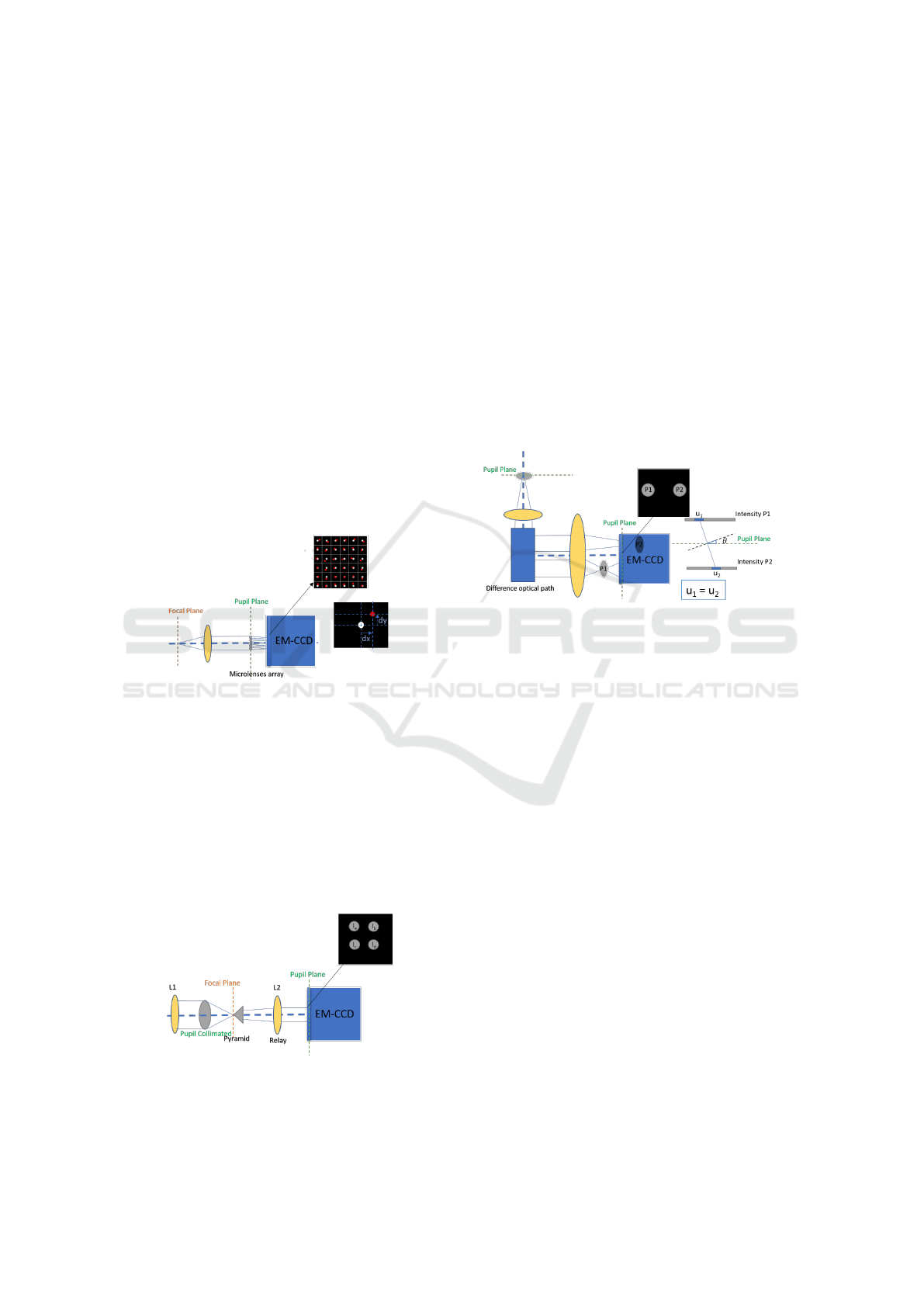
The S-H WFS was developed in the late 1960s,
evolving from the Hartmann screen test (Thibos,
2000). It works by subdividing the complex field in
the plane of the telescope’s pupil, the hardware part
is a lenslet array that generates low resolution images
of the object. See figure 1. The integrated gradient of
the wavefront across the lenslet is proportional to the
displacement of the centroid (dx,dy). Consequently,
any phase aberration can be approximated by a set of
discrete tilts.
Figure 1: Shack-Hartmann WFS scheme.
The nm-PYR WFS was first introduced in 1996
by Ragazzoni (Ragazzoni, 1996). For this sensor the
hardware part is a pyramid, which is placed on the fo-
cal plane of the telescope and the light is focused on
the apex of the pyramid. This element subdivides the
focal plane of the telescope into four quadrants. The
output of the prism is collimated obtaining four aper-
ture images in the focal plane of the lens. From the
intensity distribution in the four pupils we can calcu-
late local slopes.
Figure 2: Pyramid WFS scheme.
The TP3 WFS was conceived by van Dam and
Lane in 2002, and was first used in a closed-loop AO
system in 2017 (Colodro-Conde and others., 2017).
It is based on the derivation of the wavefront aberra-
tions from two defocused intensity images (van Dam
and Lane, 2002). For this sensor the hardware part
will be an optical element which generates an optical
path difference. It working principle is based on the
divergences and convergences of the rays in an aber-
rated WF, which create fluctuations intensity maps.
The total intensity must be constant between the ray
path due to the principle of conservation of energy.
Thus, an area of light divergent in one image will have
the same total intensity as its respective convergent
area in the other image. The ray tracing is performed
by measuring the displacement of the corresponding
light and dark regions in the defocused images, see
figure 3.
Figure 3: Two Pupil Plane WFS scheme.
This paper presents the first work carried out to
determine the best WFS to couple ALIOLI to differ-
ent scientific instruments in medium-sized telescopes.
The final purpose is to develop simulations, labora-
tory tests and telescopic operation of a prototype that
offers the possibility of using one type or another ac-
cording to the observing conditions.
2 MODULAR CONCEPT
The ultimate purpose of this project is to have a
portable instrument that could be mated and removed
in different telescopes. For this reason, a modular sys-
tem has been proposed. The modules in the ALIOLI
instrument are as follows:
• Telescope Simulator. An optical fiber has been
used as a reference star. This block has been ini-
tially developed for the TCS. To simulate the TCS
aperture, two achromatic doublets and a physical
pupil have been used. See Figure 4 blue beam.
• Wavefront Corrector. This block consisting of a
DM placed on the conjugated pupil plane of the
telescope that act as a phase modulator. It was
decided for the simplest design using commercial
achromatic doublets. The collimating lens images
PHOTOPTICS 2022 - 10th International Conference on Photonics, Optics and Laser Technology
18
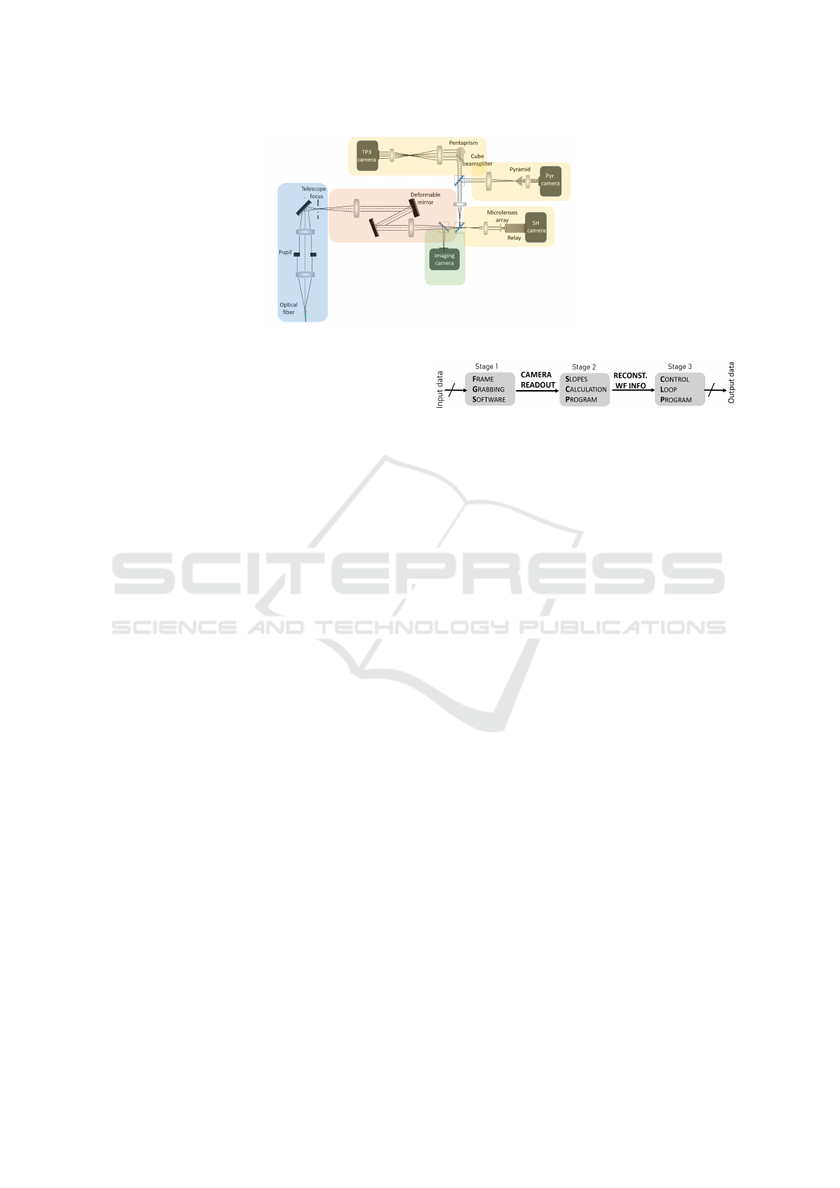
Figure 4: Mounting proposals for each module of the ALIOLI instrument.
the entrance pupil on the DM, and a second lens
refocuses the object. The DM is an ALPAO de-
vice with 88 actuators and a pupil diameter of
20mm. This compact design will allow to incor-
porate a Tip Tilt Mirror (TTM) along the optical
path, but due to the tip/tilt stroke of this DM is
40µm, in the actual design the tip-tilt corrections
could be assumed by the DM. See Figure 4 red
beam.
• Wavefront Sensor. A WFS with interchangeable
S-H, TP3, PYR modules. The optical design for
each wavefront is done and it is widely reported
in Section 3. The sensor camera, an Andor Ixon
DU-897 camera, which is based on a sub-photon
noise 512x512 e2v EMCCD (Electron Multiply-
ing Charge-Coupled Device) detector, and the col-
limating lenses are common for the three ap-
proaches. See Figure 4 yellow beam. Each WFS
carries an image analysis program for calculat-
ing the slopes, Slopes Calculation Program (SCP),
that reproduce the incident wavefront.
• Control Software. The same modular strategy
has been proposed for the Control Software. See
Figure 5. Here, we will distinguish three mod-
ules. The first one is the Frame Grabbing Soft-
ware (FGS) whose objective is to continuously
acquire images from the WFS camera, the input
data, using an appropriate configuration depend-
ing on the post processing. This part send the
images to the next level. The second ones is the
Slope Calculation Program (SCP) which receives
the images and processes them according to each
algorithm. The information collected after pro-
cessing is sent in terms of slopes or Zernike coef-
ficients to the next level. The last module is the
Control Loop Program (CLP). The base of this
prototype is to use resources of previous projects,
so the CLP used is the one developed for AOLI,
whose description is widely reported in (Colodro-
Conde and others., 2017).
Figure 5: Pipeline for the Analysis + Control Software.
• Graphics Manager. A python application has been
developed to manage the graphics produced dur-
ing the AO process, such as the reconstruction of
the wavefront, the DM geometry or the WFS cam-
era readout. This application allows view real-
time information relevant to the sensing and close
loop process, as well as save the information in
the appropriate format.
• A Science System: the initial approach is to place
directly an imaging camera. Since our WFC
maintains the telescope’s F#, we have decided to
attach the lenses of FastCam instrument, based
on Lucky Imaging technique, (Alejandro Oscoz,
2008) to our science arm. See Figure 4 green
beam. Using an adaptive optics system prior
to a lucky imaging detector, first tested in 2007
(Gladysz et al., 2007), allows obtain a higher
number of images minimally affected by turbu-
lence. The lucky imaging system averages the
best images taken during the AO process to get a
final image with higher resolution than it is possi-
ble with a regular long exposure AO camera. The
EMCCD camera is an iXon 888 from Andor, with
sensor diagonal size 18.8 mm and pixel size 13
µm.
3 WAVEFRONT SENSORS
DESIGN
Throughout this section we will explain the design
of each one of the wavefront sensors, at the concept
level, the selection of the optical components as well
as the outlook of the Slopes Calculation Program.
Study of Three WFS for the Modular System in a Portable AO Instrument: ALIOLI
19

3.1 Shack Hartmann
In the operation of a wavefront sensor type SH there
are three basic steps in the analysis process: determi-
nation of the spot positions, conversion to wavefront
slopes, and the wavefront reconstruction.
In the design, the deformable mirror and the mi-
crolenses array (MA) are in a pupil conjugate plane,
we are looking for the simplest setup, so our choice
was to select a commercial MA. The first design was
carried out using the MLA300-14AR(-M) Thorlabs
model Square Grid with size 10mm x 10mm and
lenslet pitch 300µm.
The higher the number of lenslets sampling the
pupil, the higher is the spatial resolution of the mea-
surements. However, this will lead to a lower sig-
nal to noise ratio since we reduce the amount of light
by lenslet, so we have to find a balance between
these two parameters. Our idea is to control the sam-
pling varying the pupil size over the MA, and this
is achieved by modifying the collimation lens that
projects the pupil on the MA.
We need to know the minimum number of mi-
crolenses required to accurately sample the tele-
scope’s pupil. The seeing for a good night at the TCS
in the Teide Observatory is r
0
= 0.15m. Therefore,
the area of the telescope’s pupil must be divided by
the area of the atmospheric cell to know the regions in
which our pupil has to be divided and, consequently,
the minimum number of microlenses across our pupil:
Number of regions =
(1.52)
2
(0.15)
2
∼ 103 regions.
Two different designs have been tested. The first
one assumed a 5.4mm pupil, and therefore an over-
sampling of 20 x 20 microlenses. The results obtained
both in laboratory and in the telescope are summa-
rized in (Soria et al., 2020).
To improve the signal per microlense a second design
was proposed. In this case we generate a pupil of 3.6
mm and therefore an sampling of 12 x 12 microlenses.
The configuration of the detector camera is configured
to read only the area in which the light falls, to reduce
the sampling time.
A reference image whose spots falls in the cen-
tre of the microlenses areas is needed. To obtain this
image, a reference beam is inserted placing an opti-
cal fiber in the focus of the telescope (Telescope Fo-
cus Figure 4). In this configuration, the only optical
element that can introduce aberrations in the system
is the DM, since without voltage the surface is not
flat. For flattening, a commercial wavefront sensor
(Thorlabs WFS40-7AR) placed after the collimating
lens of the WFS beam. The readout has been con-
nected to the control system and after the Static Char-
acterization we have closed the loop and therefore the
DM surface has been corrected until obtaining a flat
wavefront. This flattening can be verified with the
science image in the event that both optical paths are
equal, if not, the dreaded Non Common Path Aber-
ration (NCPA) will appear. This wavefront will be
our objective readout throughout the test. This step is
common for all the WFS.
3.2 Pyramidal
The operating principle of our Pyramidal WFS consist
of focusing the distorted WF on the vertex of a pyra-
mid by L1 and split into four beams by four facets of
pyramid, and then four conjugated images of the pupil
are produced on the detector camera by L2, see figure
2. I1, I2, I3 and I4 denote their respective intensity.
For the optical design, the PAM2R.dll dynamic
linked library that define a user surface for ZEMAX
has been used as a resource, describing a pyramid
as an optical element for geometrical ray-tracing pur-
poses developed by Arcetri (Antichi et al., 2016). One
of the main problems in the manufacture of a pyra-
mid by polishing is the roof-shaped tip, especially for
small angles, which produce not evenly spread into
four parts. The angle is limited by the area of the de-
tector so two different pyramids have been proposed.
A simple one with a base angle of 8 degrees, and a
double one with 20 and 12 degrees. The use of a dou-
ble pyramid allows to select a base angle greater than
with a single pyramid configuration which results in
an easier polishing process (Tozzi et al., 2008b). Nev-
ertheless, because of the higher thickness, it creates
another problem: the appearance of chromatic aber-
ration. For this reason, a design with two different
glasses is needed (Tozzi et al., 2008a). Both pyramids
are still in the design process.
Due to the group’s lack of experience with this
sensor, the Slope Calculation Program will have to be
developed. To date, the algorithm has been verified
through different simulations, but it must be imple-
mented in real time, and its output must be compatible
with our Control Loop Program.
3.3 Two Pupil Plane Positions
This was the WFS used in the previous instrument
AOLI. For this task, the optical design had to be
changed because a much more compact instrument is
needed, so to generate a sufficient difference in the
optical path it was not possible to use a Lateral Prism.
There are two Lateral Prisms available: 10mm and
20mm. The large one induces an excessive separa-
tion of the pupils on the detector, while the smaller
PHOTOPTICS 2022 - 10th International Conference on Photonics, Optics and Laser Technology
20
one generates an optical path difference less than the
depth of focus of the telescope, so the selected optical
element to introduce the optical difference path is a
pentaprism.
As we have mentioned, the greater the projection
of the wavefront, the greater the resolution of our sen-
sor, so the difference in the optical path that we intro-
duce is proportional to it. This optical element in-
duces two potential problems, the decrease in the in-
tensity due to the absorption of the pentaprism and the
inversion in the pupil. Therefore, some adjustments
have been made in the slope calculation program. To
solve the problem related to the differences in the il-
lumination, it is carried out a normalization of each
pupil, and for the inversion a X-flip is done in one of
the pupils before applying the algorithm.
The steps to apply the Van Damm algorithm are ex-
plained in the simulation section. The real time SCP
works in real time thanks to its GPU-accelerated im-
plementation (Fern
´
andez-Valdivia et al. 2013)
4 PYTHON SIMULATIONS
We have been developing simulators for the 3 WFS
to test the algorithm of each SCP. This study helps
us better understand our system and be able to make
sensor comparisons in a theoretical way. To carry out
the simulations we used Python as programming lan-
guage.
The setup components have been simulated using
the High Contrast Imaging for Python (HCIPy) mod-
ule developed by a group of astronomers at Leiden
Observatory (Por et al., 2018), see table 1.
The phase profile of the deformable mirror
ψ
DM
(x, y) can be described by two different ways:
through a Gaussian profile of influence of each ac-
tuator c
act
or set of modal functions f
i
(x, y) defined
by:
ψ
DM
(x, y) =
∑
i
c
i
f
i
(x, y) (1)
Modal reconstruction involves the estimation of
the actuator state c
act
or the modal coefficients c
i
that
compensate the incident aberration. Throughout this
paper, the actuator modes will be used in Zernike
mode.
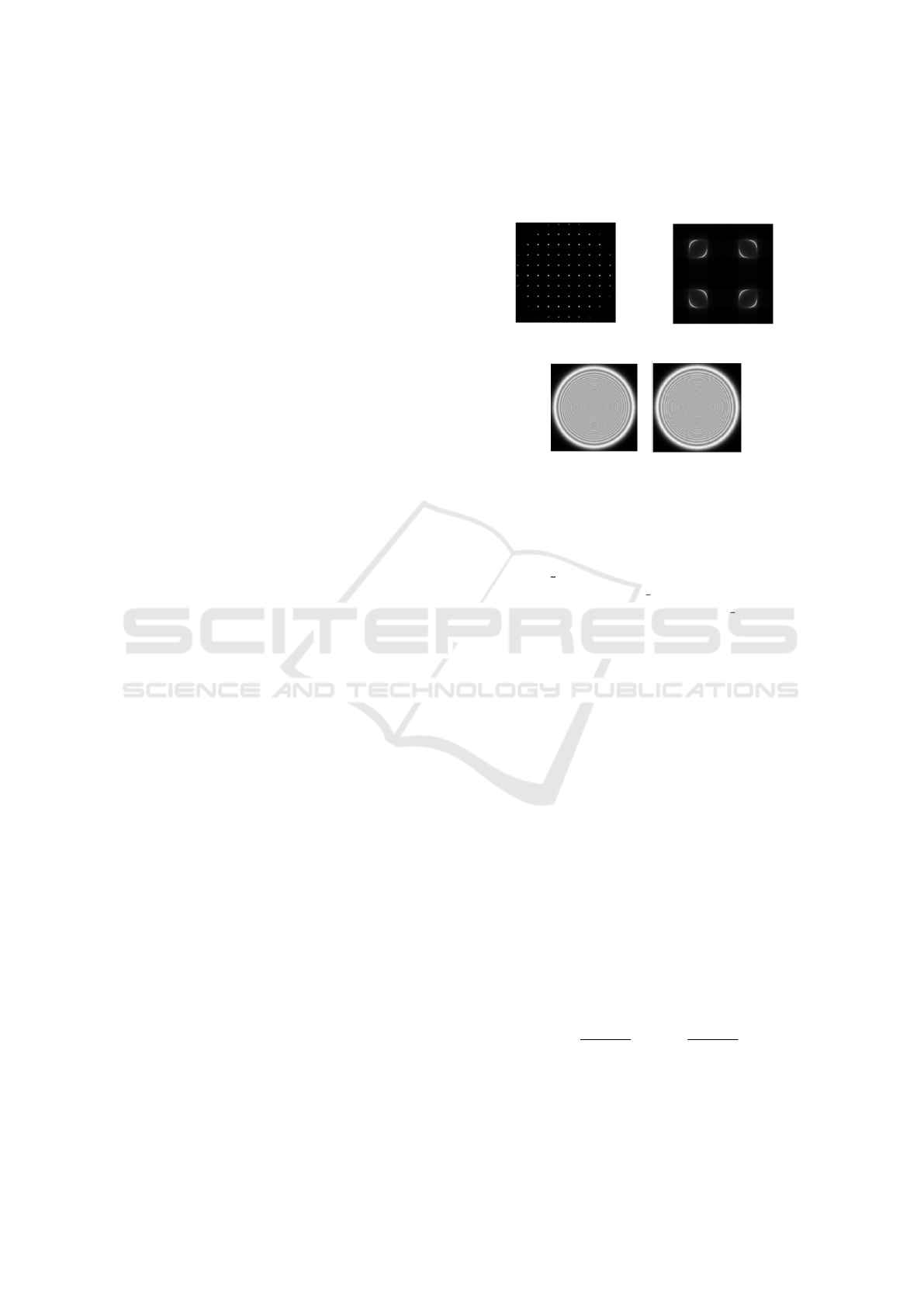
For the reference image, the DM is flattened and
a perfect flat wavefront that passes through the pupil
of the telescope is generated. This WF passes through
the different components, the pupil reducer, the DM
and the different optical elements of each WFS, mi-
crolenses array (MA) for the SH, the pyramid for the
PYR and 2 Fresnel propagator surfaces for the TP3.
After that, the signal is read on the detector camera
and the image is normalized. Once the camera is
read out, each image is analysed though functions that
carry out the algorithms explained in the section 3.
(a) Reference image for the
SH.
(b) Reference image for the
Pyr.
(c) Reference image for the TP3.
Figure 6: Reference image for each WF.
For the SH, the simulation of the MA is defined
though the HCIPy function:
MicroLensArray(pup_grid,mla_grid,focal_length)
Where pup grid defines the area in which the light
will fall over the MA, mla grid defines the positions
of the centre of the micolenses, and focal length is the
value of the focal of the microlenses.
We use the reference image to select the lenslet
area in which to measure each centroid (microlens
pitch) and the ideal position of the spots, in the case
of the simulation this points will be the same that the
coordinates that define the pupil grid, see Figure 6a.
To carry out this task we have implemented a func-
tion that from an input value of the spots distance,
that we mark over the reference image, it performs a
peak detection algorithm, and in the last iteration it
saves the position of the centroid of each microlens
and the parameter that characterize the readout area.
This method allows us to apply the algorithm to dif-
ferent assemblies that we could use. From the refer-
ence we generate a mask that selects the areas of the
detector in which the software has to measure the po-
sition of the centroids. To know which pixels we have
to take into account, in this point, we apply a dynamic
threshold which is proportional to the maximum pixel
value in the cell. The localization of the spot behind
each lenslet area is determined using a centre of mass
algorithm. The x and y location are given by:
C
x
=
∑
N
i=1
x
i
l
i
∑
N
i=1
I
i
, C
y
=
∑
N
i=1
y
i
l
i
∑
N
i=1
I
i
. (2)
This calculus are involve in the following imple-
mented function:
SH_estimator(det,regx,regy,regh,regw,refx,refy)
Study of Three WFS for the Modular System in a Portable AO Instrument: ALIOLI
21

Table 1: Characteristics of simulated elements.
Parameter Value
Telescope Diameter 1.5 m
Pupil diameter over the DM 18.11 mm
WFS Wavelength 700 nm
SH: Subapertures 12 x 12
SH: Focal 14.6mm
SH: Lenslet diameter 300 µm
Pyramid separation 0.04
TP3 optical path difference 10mm
DM: Actuators across pupil 9
DM influence Zernike polynomails
Science camera Noiseless detector 1024 x 1024 px
WFS camera Noiseless detector 256 x 256 px
Number of Zernike reconstruct coefficients 30
Being det the image we want to process, and the rest
of the inputs the parameters that mark the readout
area.
From that moment, the SCP will measure the position
of the centroids in each of the regions that we have
defined on the detector and will compare the results
with those of the reference image to calculate the dis-
placements in x and y for each subaperture.
For the PYR WFS the pyramid is simulated
though the HCIPy function:
PyramidWavefrontSensorOptics(pupil_grid,sep,wl_0)
Where pup grid defines the area in which the light
will fall, sep, separation, is related to the angle of
the pyramid root, and wl 0 is the wavelength used for
sensing. To know the detector readout area, we have
implemented a circle detection function:
Detect_circle(direction_image,minR,maxR)
Where direction image point to the folder where the
reference image has been saved, and minR,maxR de-
limit the expected range of the radius of the circle we
are looking for in pixels. This function applied an
Hough filter to the binarized reference image using
the OpenCV library, and it returns the x and y coordi-
nates of each detected circle and its radius. Using this
parameters we could create a square mask that extract
the pixel values of the detector which correspond to
the pupils areas. To avoid edge effects, that we have
verified to have a great weight in the reading of the
WF, the readout area is 2 pixel smaller than the size
of the detected circle. This approach allows operate
with the pupils as simple matrices. Finally, we apply
the algorithm to calculate the deviations in the x and
y direction:
I
x
=
(I
a
+ I
b
−I
c
−I
d
)
norm
(3)
I
y
=
(I
a
−I
b
−I
c
+ I
d
)
norm
(4)
The normalization factor could be calculated using
different methods (Bond et al., 2015). For this ap-
proach we have chosen the classical normalisation for
a pyramidal WFS, a pixel-wise normalization. Ev-
ery pixel intensity is normalised by the total intensity
in that pixel position, summed across the four pupils.
The algorithm has been implemented in the function:
Proc_pupil(aberr,pupils)
Where aberr is the detector frame that we want
to analyse, and pupils contains the information re-
garding the areas of the detector that we have to
read, namely, the output of the previous function
Detect circle.
In the case of the TP3 WFS, the optical path dif-
ference between the pupils has been generated adding
to the beam two Fresnel surfaces defined in the HCIPy
library:
F1=FresnelPropagator(pupil_grid,z,num_oversamp,n)
F2=FresnelPropagator(pupil_grid,-z,num_oversamp,n)
Once again pupil grid marks the area in which the
light will fall, z is half of the distance generated be-
tween the pupils, oversamp is the number of times the
transfer function is oversampled, and n is the refrac-
tive index in which the light spreads. To simplify the
process each pupil is read out in its own detector, so it
is not necessary to extract the pupils. We use the ref-
erence image to delimiter the size of the pre-calculus
polynomial slopes matrix and the coefficients read for
the reference image are used as a baseline. Figure
6c. Following the Vam Dam article, the first step is to
calculate the mean slope of the polynomials in the or-
thogonal direction to the projection. For every angle,
α, and a circle of radius R this quantity is given by:
H
α
(u, Z
y
) =
1
2
√
R
2
−u
2
× .
R
∂Z
t
(x, y)
∂x
cos(θ) +
∂Z
t
(x, y)
∂y
sen(θ)
(5)
PHOTOPTICS 2022 - 10th International Conference on Photonics, Optics and Laser Technology
22

Being R the Radon Transform and u the coordinates.
The calculation of the Radon Transform has been
implemented in python based on the code of Justin
K. Romberg, making a small modification so that
it returns the reference coordinates of the calculated
sinogram, that we need to use in this algorithm.
The derivatives of the Zernike polynomials can be
computed directly from their mathematical definition.
These calculations have been implemented within the
following function:
H = g_wfs_precalc(modes, angles, x, y)
Whose inputs are modes, a vector with the modes
used for the reconstruction, angles a vector with the
projection angles for the Radon Transform, and the
horizontal size, x, and vertical size, y, of the readout
area. This function returns a 3D matrix H whose size
is H[number of coords, number of angles, number of
modes.
The Zernike coefficients a
i
are then calculated
through a least squares fit:
a
i
= [Hα(u, Z
i
)
T
H
α
(u, Z
i
)]
−
1H
α
(u, Z
i
)
T
p
α
(u) (6)
Being [Hα(u, Z
i
)
T
H
α
(u, Z
i
)]
−
1H
α
(u, Z
i
)
T
the expres-
sion of the Moore-Penrose pseudo-inverse, a general-
ization of the inverse. The first step is to convert our
3D matriz in an 2D matrix to operate with it, for this
task a simple reshape was applied. The second step
is to carry out the pseudoinverse. To avoid degrada-
tion of the reconstruction by small singular values, we
have used the Thicknov regularization that is imple-
mented in the HCIPy library. We choose a tolerance
of 10
−3
.
The next step is to calculate the sinogram, by
means of the Radon transform, of each of the unfo-
cused pupils, and then relate the intensities by means
of an histogram matching. Once I know the coordi-
nates of each sinogram that have the same light in-
tensity (u
1
and u
2
), I can calculate the slope of the
incident wavefront by:
∂W
r∂u
=
u
1
−u
2
2 ·z
(7)
Finally, to calculate the slope along the pupil we
have to perform an interpolation of the measured val-
ues. The function chosen to carry out the interpolation
has been InterpolatedUnivariateSpline from Scipy li-
brary. All these calculations have been implemented
within the following function:
g_wfs(i1, i2, nangles, z ,H_pinv)
Where i1 and i2 are the detector images of each blur
pupil, nangles the number of angles projected, z the
distance in meters between each pupil and the pupil
focus plane, and H pinv the pseudo-inverse of the H
matrix. This function returns the slopes calculated
if H pinv is NONE or otherwise the reconstructed
Zernike coefficients.
Up to here we would have completed the simula-
tion of the WFS module, the next phase will be the
simulation of the calibration of our instrument.
For the linear reconstructor we need to now the
Influence Matrix, which tells us how each wavefront
sensor responds to each movement of the deformable
mirror. We are working in Zernike mode basic for
the DM characterization so the modal characteriza-
tion can be build by sequentially applying a positive
and negative single mode on the deformable mirror
surface and reading the measurement on each WFS.
The difference between the two WFS readouts gives
us the DM response. The most common technique
of wavefront reconstruction is to assume a linear rela-
tion between the measurement vector s and the modal
coefficients c. The forward model is then given by:
s = M
in f lu
·c + N (8)
Where M
in f lu
is the Influence Matrix, s the WFS mea-
surement, c the incoming perturbation and N some
measurement noise from the WFS. The Influence Ma-
trix can be calibrated by measuring the actuator re-
sponse within the linearity range of the WFS. The
inverse operation of reconstructing the WF from the
slope measurements involves the estimation of the
Actuation Matrix, M
act
. This estimation requires in-
version of the Influence Matrix. M
in f lu
is not a square
matrix so to apply the least-squares a pseudo-inverse
in needed. Again we use the pseudo-inverse of Thic-
knov.
For each WFS we have implemented a function
responsible of calculate M
in f lu
. In addition to the re-
quested parameters that characterize each WFS oper-
ation, there are some common inputs that indicates the
number of DM actuators poke, the number of mea-
surements and the number of modes that we apply to
the DM.
Once we have completed the calibration process,
we could reconstruct the shape of the incoming WF
just multiplying the WFS lecture by the Actuation
Matrix:
c = M
act
·s (9)
4.1 Results
As our objective is to verify the reliability of the algo-
rithm under different conditions, it is more useful to
generate a controllable wavefront and check whether,
after the analysis and reconstruction, the wavefront
corresponds to the simulated one. It is a static mea-
surement, so for simplicity we are going to resort
leaving the deformable mirror in a random position
and checking the reconstruction of its surface with
each of the sensors. The results are shown in figures
7, 8 and 9:
Study of Three WFS for the Modular System in a Portable AO Instrument: ALIOLI
23
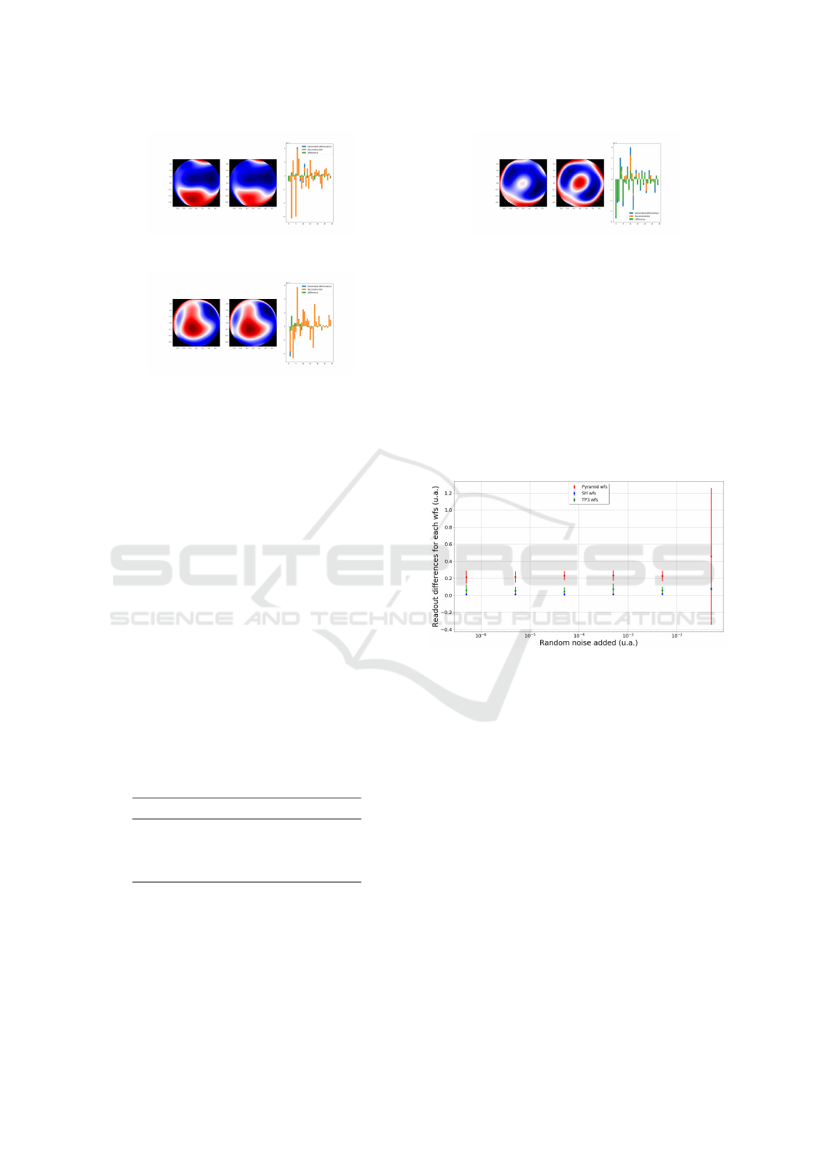
Figure 7: Reconstruction process for the SH module simu-
lation.
Figure 8: Reconstruction process for the TP3 module simu-
lation.
The first image shows the DM surface when we
send it a random signal, the second shows the recon-
struction of the WF with each WFS, and the third
figure shows an histogram with the generated modes
(blue), the reconstructed modes (orange), as well as
the difference between them (green).
On first thought, if we compare the first and the
second figure, we see as the reconstruction algorithm
used for the SH WFS and the TP3 WFS reconstruct
the incident wavefront in a more faithful way than the
algorithm used with the nm-PYR module showing the
non-linear behaviour of this sensor referenced in the
bibliography (Hutterer et al., 2019).
For a statistic study, we generate 90 random positions
for the DM, working with 30 Zernike coefficient and
leaving aside the mode 0 corresponding to the pis-
ton. Then, we perform the reconstruction process
with each WFS and calculate the Root Mean Square
(RMS) of the difference vector. Results obtained are
summarized in table 2.
Table 2: Differences between the incoming WF and the re-
constructed WF for each WFS.
RMS (u.a.)
SH wfs (1.58 ±0.03) ·10
−02
Pyr wfs (2.1 ±0.6) ·10
−01
TP3 wfs (5 ±4) ·10
−02
In the absence of noise, the goodness of the re-
construction process differs by an order of magni-
tude between the PYR WFS and the others. SH WFS
shows better results, with the smallest RMS. More-
over, the error associate to the RMS measurement in-
dicates that the SH WFS is more precise.
To analyse the behaviour of the sensors under real
Figure 9: Reconstruction process for the Pyr module simu-
lation.
conditions, we are going to carry out a study of the
reconstruction process when the input signal is not
clear. For this task we are going to add random noise
to the detector camera, whose medium value is zero
and the Standard Deviation (SD) will vary. This sit-
uation would reflects the observation with different
reference stars magnitudes. The results in Figure 10
summarize the performance of the sensors, and error
bars show the SD (over maximum and minimum val-
ues) of the measured RMS value for each noise value.
See figure 10.
Figure 10: WFS response comparison for different SN ra-
tios.
The same trend is followed when the measure-
ments have noise. The high SD for the PYR WFS
in the last point shows that this WFS is not capable
of reconstruct the incident WF under this conditions
while the SH and the TP3 get good results.
5 CONCLUSIONS
In the WFS comparison there are many requirements
that we have to balance for the AO system design.
• Accuracy
• Efficiency (good use of photons)
• Speed (related with linearity)
• Robustness (chromaticity, ability to work on ex-
tended sources, etc ...)
• Other parameters (price, assembly-friendly..)
PHOTOPTICS 2022 - 10th International Conference on Photonics, Optics and Laser Technology
24

These simulations have given us the chance to test
the implemented algorithm for the three WFS. Results
show that the SH WFS is the most accurate and pre-
cise. The same efficiency has been obtained for the
TP3 and the SH WFS.
Other requirements such as speed will have to be
rated when the real time implementation will be fin-
ished for the three WFS. To compare others parame-
ters specific test will be designed.
Furthermore, these simulations have allowed us to
discard the nm-PYR for our instrument, opening the
possibility of design a modulated one to increase lin-
earity.
ACKNOWLEDGEMENTS
The research leading to these results received the sup-
port of the Spanish Ministry of Science and Inno-
vation under the FEDER Agreement INSIDE-OOCC
(ICTS-2019-03-IAC-12) and managed by the Insti-
tuto de Astrof
´
ısica de Canarias (IAC).
REFERENCES
Alejandro Oscoz, a. o. (2008). FastCam: a new lucky
imaging instrument for medium-sized telescopes. In
McLean, I. S. and Casali, M. M., editors, Ground-
based and Airborne Instrumentation for Astronomy II,
volume 7014, pages 1447 – 1458. International Soci-
ety for Optics and Photonics, SPIE.
Antichi, J., Munari, M., Magrin, D., and Riccardi, A.
(2016). Modeling pyramidal sensors in ray-tracing
software by a suitable user-defined surface. Journal of
Astronomical Telescopes, Instruments, and Systems,
2(2):1 – 7.
Bond, C., El Hadi, K., Sauvage, J. F., Correia, C., Fau-
varque, O., Rabaud, D., Neichel, B., and Fusco, T.
(2015). Experimental implementation of a Pyramid
WFS: Towards the first SCAO systems for E-ELT. In
Adaptive Optics for Extremely Large Telescopes IV
(AO4ELT4), page E6.
Colodro-Conde, C. and others. (2017). Laboratory and tele-
scope demonstration of the TP3-WFS for the adaptive
optics segment of AOLI. Monthly Notices of the Royal
Astronomical Society, 467(3):2855–2868.
Colodro-Conde, C. and others. (2018). The TP3-WFS: a
new guy in town. page arXiv:1811.05607.
Gladysz, S., Christou, J. C., and Redfern, M. (2007). “lucky
imaging” with adaptive optics. In Adaptive Optics:
Analysis and Methods/Computational Optical Sensing
and Imaging/Information Photonics/Signal Recovery
and Synthesis Topical Meetings on CD-ROM, page
ATuA7. Optical Society of America.
Hickson, P. (2014). Atmospheric and adaptive optics. The
Astronomy and Astrophysics Review, 22:1–38.
Hutterer, V., Ramlau, R., and Shatokhina, I. (2019). Real-
time adaptive optics with pyramid wavefront sensors:
part i. a theoretical analysis of the pyramid sensor
model. Inverse Problems, 35(4):045007.
Por, E. H., Haffert, S. Y., Radhakrishnan, V. M., Doel-
man, D. S., Van Kooten, M., and Bos, S. P. (2018).
High Contrast Imaging for Python (HCIPy): an open-
source adaptive optics and coronagraph simulator. In
Adaptive Optics Systems VI, volume 10703 of Proc.
SPIE.
Ragazzoni, R. (1996). Pupil plane wavefront sensing with
an oscillating prism. Journal of Modern Optics,
43(2):289–293.
Soria, E., L
´
opez, R. L., Oscoz, A., and Colodro-Conde,
C. (2020). ALIOLI: presentation and first steps. In
Schreiber, L., Schmidt, D., and Vernet, E., editors,
Adaptive Optics Systems VII, volume 11448, pages
517 – 525. International Society for Optics and Pho-
tonics, SPIE.
Thibos, L. N. (2000). Principles of hartmann-shack aber-
rometry. In Vision Science and its Applications, page
NW6. Optical Society of America.
Tozzi, A., Stefanini, P., Pinna, E., and Esposito, S. (2008a).
The double pyramid wavefront sensor for lbt. In Hu-
bin, N., Max, C. E., and Wizinowich, P. L., editors,
Adaptive Optics Systems, volume 7015, pages 1454 –
1462. International Society for Optics and Photonics,
SPIE.
Tozzi, A., Stefanini, P., Pinna, E., and Esposito, S. (2008b).
The double pyramid wavefront sensor for LBT. In
Hubin, N., Max, C. E., and Wizinowich, P. L., editors,
Adaptive Optics Systems, volume 7015, pages 1454 –
1462. International Society for Optics and Photonics,
SPIE.
van Dam, M. A. and Lane, R. G. (2002). Wave-front sensing
from defocused images by use of wave-front slopes.
Appl. Opt., 41(26):5497–5502.
Study of Three WFS for the Modular System in a Portable AO Instrument: ALIOLI
25
