Surface Light Barriers
Theo Gabloffsky
a
, Britta Kruse and Ralf Salomon
University of Rostock, 18051, Germany
fi
Keywords:
Light Barrier, Neural Network, Backpropagation Network, Radial Basis Function, Speed Measuring, Curling.
Abstract:
It should be known to almost all readers that light barriers are commonly used for measuring the speed of
various objects. These devices are easy to use, quite robust, and of low cost. Despite their advantages, light
barriers exhibit certain limitations that occur when the objects of interest move in more than one spatial dimen-
sion. This paper discusses a physical setup in which light barriers can also be used in case of two-dimensional
trajectories. However, this setup requires rather complicated calculations. Therefore, this paper performs these
calculations by means of different neural network models. The results show that backpropagation networks as
well as radial basis functions are able to achieve a residual error less than 0.21 %, which is more than sufficient
for most sports and everyday applications.
1 INTRODUCTION
In modern sporting events, technology is present
in numerous applications, for example in scoring
boards, video proof, or just for measuring distance
and time in competitions. In addition, regular prac-
tice is interested in recording and analyzing physical
data, in order to enhance performance. These phys-
ical data can be manifold, for example time, weight,
speed, and distance.
However, the recording of the speeds of objects
and athletes can be considered of special interest in
various sports, such as bobsleigh, tennis, and run-
ning. From a physics point of view, an object’s speed
v = ∆s/∆t is defined as the distance ∆s it travels
during the time interval ∆t. Commonly used speed
measuring technologies include RFID transponders,
wearable GPS devices or a video-based tracking. An-
other tool for measuring the speeds of objects are
light barriers which are comparatively simple, suffi-
ciently precise, and easy to install. As shown in Fig.
1, a light barrier basically consists of three compo-
nents, a light source, a sensor, and an evaluation unit.
The first two elements are aligned in a way that the
light source projects onto the sensor. If a moving
object travels through the light barrier, the beam of
light is interrupted, which is recognized by the eval-
uation unit, which in turn generates a timestamp t
1
.
With two light barriers in place, the speed v reads:
v = (x
2
− x
1
)/(t
2
−t
1
) = ∆x/∆t.
a
https://orcid.org/0000-0001-6460-5832
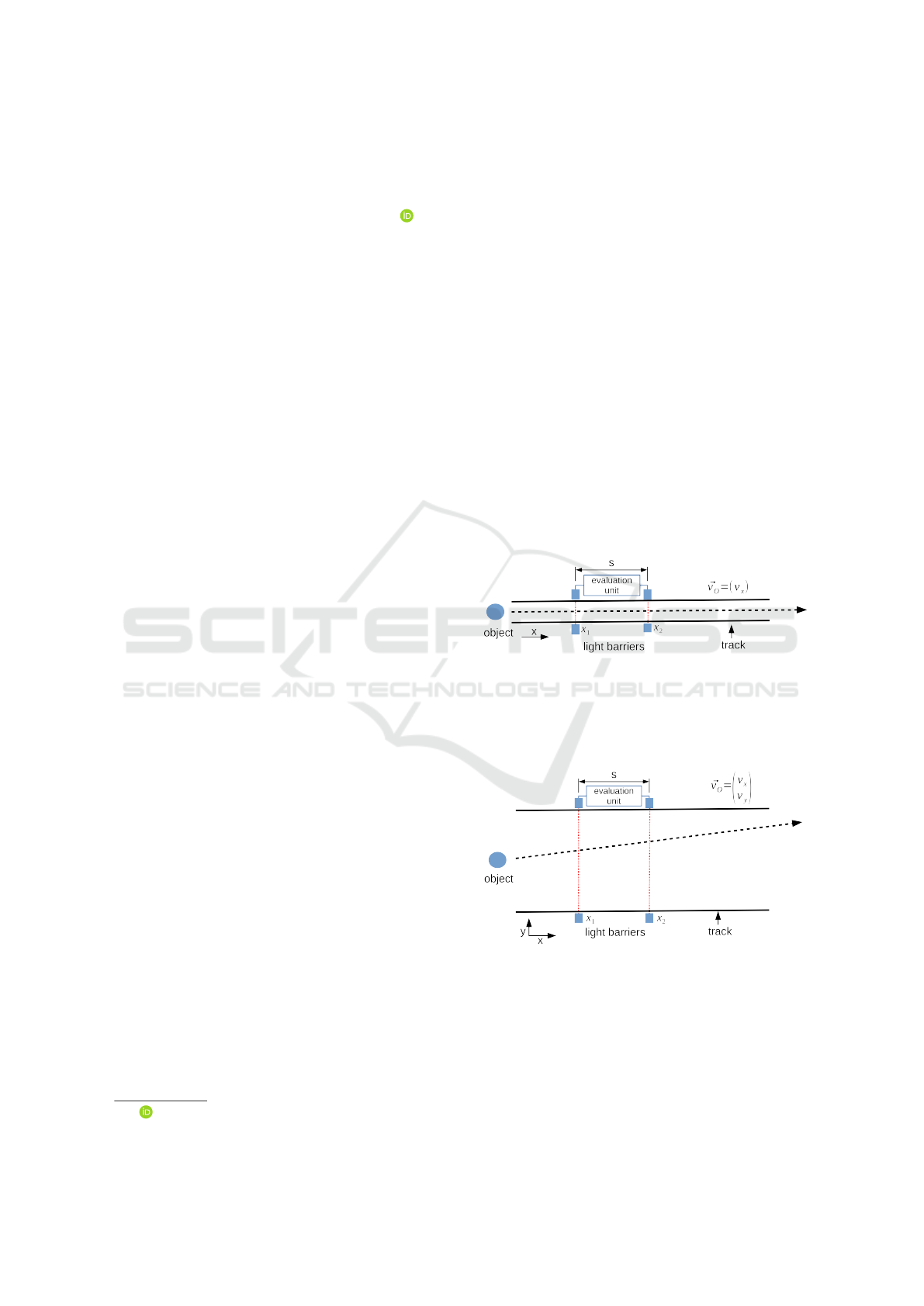
Figure 1: Usually two light barriers are used to measure
the speed of an object that is moving in a narrow path. On
crossing a beam of light, the respective light barrier records
a timestamp t
i
. With two timestamps t
1
and t
2
and the trav-
eled distance s, the resulting speed is v = (t
2
− t
1
)/s. The
computations are done by the evaluation unit.
Figure 2: The physical setup shows the possible path of the
object through a wide path. Here, an object can move in the
x-direction and also in the y-direction. Thus, the velocity
⃗v = (v
x
,v
y
)
T
is a two dimensional vector.
The examples mentioned above are simple by
their very nature: the moving direction is always
along the physical environment, and thus perpendic-
ular to the orientation of the light barriers. There-
fore, both speed v and velocity are identical quantities
Gabloffsky, T., Kruse, B. and Salomon, R.
Surface Light Barriers.
DOI: 10.5220/0010777500003118
In Proceedings of the 11th International Conference on Sensor Networks (SENSORNETS 2022), pages 97-104
ISBN: 978-989-758-551-7; ISSN: 2184-4380
Copyright
c
 2022 by SCITEPRESS – Science and Technology Publications, Lda. All rights reserved
97

v = |⃗v|.
The situation is not always as simple as described
above. For example in the sports of shot put or curl-
ing, the objects might also have a speed component
v
y
that is perpendicular to the main orientation of the
physical setup as illustrated in Fig 2. This component
might assume significant values, which invalidate the
speed measurements as given by the light barriers, at
least to some degree. In curling, for example, the
scientific support of the training process of the ger-
man national teams require the precise measurement
of both values v
x
and v
y
.
This paper presents a new light barrier system
called Surface Light Barriers (SLB), which offers a
possible solution to this problem. As Section 2 shows,
the system consists of four light barriers, which are set
up in different angles with respect to the x-direction
of the track. When an object travels through the light
barriers, the system generates four timestamps from
which it calculates the object’s two-dimensional ve-
locity ⃗v = (v
x
,v
y
)
T
. In addition, it calculates the ob-
jects starting position p = (p
x
, p
y
)
T
and end posi-
tions q = (q
x
,q
y
)
T
. Since the required calculations
are rather cumbersome, this paper explores various
neural network models. To this end, Section 3 briefly
reviews two different network models, i.e. backprop-
agation networks and radial basis functions.
For the evaluation, the neural networks were
trained with an exemplary dataset generated on the
basis of the sport of curling. The specific configura-
tions are summarized in Section 4.
The results, as shown in Section 5 and discussed
in Section 6, indicate that in terms of the average er-
ror, the best neural network is a radial basis function
network, which achieves an average error of 0.21 %.
In terms of the speed to error ratio, the best network is
a backpropagation network that employs two hidden
layers and achieves an error of 0.901%.
Finally, Section 6 concludes this paper with a brief
discussion.
2 SURFACE LIGHT BARRIERS:
PHYSICAL SETUP
As already discussed in the introduction, light barriers
face limitations in observing two-dimensional veloci-
ties when they are used in their usual setup. The Sur-
face Light Barriers system, or SLB for short, solves
this problem with a physical setup, as presented in
Fig. 3. This setup consists of the following hardware
configuration:
1. Two light barriers L1 and L4 are positioned at x
1
and x
4
and are aligned orthogonal to the main di-
rection of movement. The distance between these
light barriers is called s
2
.
2. Two light barriers L2 and L3 are positioned at x
2
and x
3
, with an alignment angle of γ ̸= 90
◦
. The
distance between these light barriers equals the
distance s
1
= s
2
/2.
3. An evaluation unit, which includes a microcon-
troller with a time tracking mechanism and a neu-
ral network.
In essence, the evaluation unit employs a micro-
controller to which every light barrier is connected via
an input port. When an object crosses a light barrier,
the interruption of the beam of light sends a signal
to the corresponding port of the microcontroller. The
microcontroller detects signal changes by either pe-
riodical polling of the input pin or the execution of
hardware interrupts.
In case of a signal change, the evaluation unit
generates a timestamp. After the object has crossed
all four light barriers, the evaluation unit has gener-
ated a total number of four individual timestamps t
1..4
.
Without loss of generality, these timestamps can also
be presented as differential quantities:
∆t
1
= t
1
−t
1
∆t
2
= t
2
−t
1
∆t
3
= t
3
−t
1
∆t
4
= t
4
−t
1
(1)
Equation (1) provides a transformation in time
such that an object enters the system at the virtual
time t = 0. It might be helpful to mention, that due
to the physical setup,
t
1
< t
2
,t
3
,t
4
always holds, and that thus all differential
quantities ∆t
i
are always positive.
3 SURFACE LIGHT BARRIERS:
NEURAL NETWORKS
The purpose of the evaluation unit is to deliver the ve-
locity⃗v , i.e., the speeds v
x
and v
y
, as well as the start-
ing and end points p
y
and q
y
of the object. However,
the mathematical approach is rather cumbersome, and
is, therefore, presented in short in the appendix. As
an alternative, this paper employs various neural net-
works for this task. It explores the utility of back-
propagation networks as well as radial basis function
networks.
Training Data: Training data are elementary for
training neural networks. Verification data are also
SENSORNETS 2022 - 11th International Conference on Sensor Networks
98

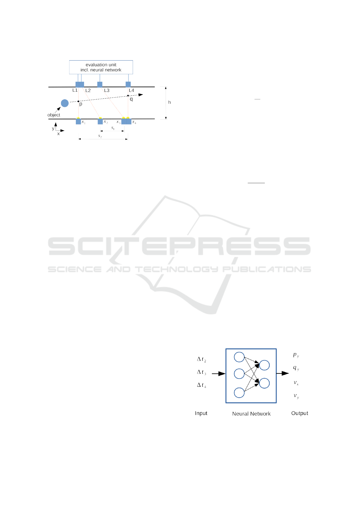
Figure 3: Example setup for the SLB-system, which basi-
cally consists of four regular light barriers and an evaluation
unit. Two of the light are arranged as usual, whereas the
other two light barriers are inclined in regard to the other
light barriers.
required for testing the generalist capabilities of the
final networks. Ideally, both datasets differ from one
another. In addition, the datasets should be drawn
such that they cover the relevant input range of the
target application.
Backpropagation Network: A backpropagation
network consists of an input layer, a choosable count
of hidden layers, and one output layer. Each layer can
consist of a different number of neurons. Every neu-
ron of a layer has weighted connections to all neurons
of the previous layer.
The output of neuron i is calculated in two steps:
(1) It calculates it net-input net
i
=
∑
n
j=1
o
j
w
i j
calcu-
lates through the summation of the outputs o
j
of the
neurons j of the previous layer. (2) It determines its
output o
i
= f (net
i
), with f (net
i
) denoting the logistic
function f (net
i
) = 1/(1 + e
−net
i
). These calculations
are done for every neuron in all hidden layers and out-
put layers.
The connections are trained with the well-known
backpropagation algorithm:
⃗w
t+1
= ⃗w
t
− η∇(⃗w
t
) (2)
For further details on backpropagation, the in-
terested reader is referred to the pertinent literature
(Wythoff, 1993).
Radial Basis Function: Radial basis functions
(RBFs) differ from backpropagation networks quite
a bit. In addition to the input layer, an RBF network
consists of only one layer of neurons. All neurons
in this layer, also referred to as kernels, maintain a
weight vector ⃗w. The vector connects each neuron
to all input neurons. In contrast to calculating the
weighted input sum, as it is done in backpropagation
networks, every neuron calculates its distance net
i
to
the current input value:
net
i
=
∑
j
(w
i j
− I
j
)
2
, (3)
Its activation θ is then set to:
θ
i
= e
net
i
β
, (4)
with β denoting a kernel width. In addition to the
weight vector ⃗w
i
, every RBF neuron also maintains an
output vector
⃗
O
i
. For the sake of simplicity, the fol-
lowing mathematical description assumes that the net-
work has only one single, scalar output value. Conse-
quently, all RBF neurons can collapse their associated
output vectors into a single output scalar O
i
. The final
network output o is then determined by applying the
softmax function:
o =
∑
i
O
i
θ
i
∑
i
θ
i
(5)
In other words, the softmax function calculates a
weighted output, which considers the target output
value O
i
of every RBF neuron as well as its current
activation θ
i
.
In many applications, all the neurons’ output val-
ues O
i
and their weight vectors ⃗w
i
are subject to
the learning process. Without loss of generality, the
SLB system assumes that all input values are possi-
ble within a given range. Thus, only the target output
value O
i
is subject to the learning process. The weight
vectors ⃗w
i
are equally distributed over the three input
domains ∆t
2..4
The SLB system applies the following
learning rule:
O
t+1
i
= O
t
i
+ (h − o
i
)ηθ
j
(6)
Every output value o
i
is adapted towards the
known target value h by an amount that is propor-
tional to the remaining difference E = (h −o
i
) as well
as the current activation of the RBF neuron θ
i
. For
further details the interested reader is referred to the
pertinent literature (Tao, 1993).
Figure 4: Overview of the input (∆t
2..4
) and output (p
y
, q
y
,
v
x
, v
y
) parameters of the neuronal network. All values are
normalized in respect to their maximum value.
Surface Light Barriers
99

4 METHODS
This section describes the datasets as well as the neu-
ral networks in full detail as far as required for the
reproduction of the results presented in Section 5.
Application Area: The SLB system has been de-
veloped as part of a project in the sport of curling.
Therefore, all key values with respect to physical
quantities, such as dimensions and speeds, have been
drawn from this project.
Simulation Hardware and Software: All mea-
surements were done on a system containing an Intel
i7 4710HQ with a clock speed of up to 3.5 GHZ and
8 GB of DDR3 RAM. The software used for simulat-
ing the networks was written in the C programming
language and no external tools were used. The simu-
lations were performed on a single core of the men-
tioned processor and no parallel calculation was used.
Dataset: The dataset was created with a mathemat-
ical model of the SLB-System including an object
which passes through the light barriers, as presented
in Fig. 3. The setup of the SLB consists of the fol-
lowing dimensions:
s
1
= 500[mm]
s
2
= 1000 [mm] (7)
h = 5 000[mm]
The trajectories of the object were generated ran-
domly bound to the following parameters:
1000 [mm/s] ≤v
x
≤ 8000 [mm/s]
−500 [mm/s] ≤v
y
≤ 500 [mm/s] (8)
0 [mm] ≤p
x
≤ 5000 [mm]
0 [mm] ≤q
x
≤ 5000 [mm]
Out of these trajectories the timestamps t
1..4
and
differential timings ∆t
2..4
were calculated. To fit
into the value range of the neural networks, the dif-
ferential times were normalized t
2..4
n
= ∆t
2..4
/t
max
by dividing each time with the longest possible oc-
curring time t
max
. This time t
max
= s
2
/v
x
min
=
1000 [mm]/1 000[mm/s] = 1 [s] is derived from the
distance s
2
between the light barriers L1 and L4 as
seen in Fig. 3 and the minimum speed of the object
v
min
= 1000 [mm/s].
The following equation describes the normal-
ization of the output parameters, where the max-
imum values depend on the generated trajectories
with respective v
x
max
= 8 000 [mm/s], p
y
max
= q
y
max
=
5000 [mm]:
v
x
n
= v
x
/v
x
max
v
y
n
= v
y
/y
y
max
(9)
p
y
n
= p
y
/p
y
max
q
y
n
= q
y
/q
y
max
In total, 10000 trajectories were created as a train-
ing set and another 1000 as a verification set. In sum-
mary, the datasets consist of the following normalized
parameters: ∆t
2
n
, ∆t
3
n
, ∆t
4
n
, v
x
n
, v
y
n
, p
y
n
, q
y
n
Naming Convention: In the following, the names
of the networks are denoted as follows: The prefix be-
fore the network name denotes the number of neurons
in the hidden layers.
As an example, the name 64-32-BP refers to
a backpropagation network with two hidden layers,
with 64 neurons in the first hidden layer h
1
and 32
neurons in the second hidden layer h
2
. The name
14-RBF refers to a radio basis function network with
14 neurons per axis, which resolves into a total of
14
3
= 2744 neurons in its neuron layer.
Backpropagation Network: The generated
datasets have been employed with different back-
propagation architectures, varied between one to
three hidden layers with four to 64 neurons in
each layer. The initial values of the weights w
i j
between the neurons were set randomly between
−0.1 < w
i j
< 0.1. The networks were trained with
a fixed learning rate of η = 0.05 and a momentum
of α = 0.9. Further information about the general
functionality of the momentum can be found in
(Phansalkar and Sastry, 1994).
All backpropagation networks utilize the
quadratic error as the loss function. The error
of a neuron j is calculated by E
j
= 1/2
∑
j
(h
j
− o
j
)
2
where h
j
is the target value of that neuron.
As the activation function, all backpropagation
networks use the logistic function: f (net) = 1/(1 +
e
−net
).
Radial Basis Function Network: The three input-
parameters are interpreted as the dimensions of the
network. Each dimension ranges from 0 to 1. Sim-
ilar to the backpropagation networks, multiple radial
basis function networks were trained. The networks
differ in the number c
dim
of neurons per dimension,
ranging from four to 20 neurons per dimension. This
results in a total of up to c
total
= c
3
dim
= 20
3
= 8000
neurons in the largest network. The distance between
the neurons is set to β = 0.1 c
dim
. The learning rate of
SENSORNETS 2022 - 11th International Conference on Sensor Networks
100

the RBF was set to η = 0.5. The error of an output
j in the radial basis function network E
j
= (h
j
− o
j
)
is equal to the absolute of the difference between the
target value h
j
of the output and the softmax of the
activation of the network o
j
.
Total Error of the Networks: The total error of a
network describes the average error of the output pa-
rameters of that network:
E
total
=
1
4
(E
p
y
+ E
q
y
+ E
v
x
+ E
v
y
) (10)
Measurement of Computational Costs: Though
the target computer-architecture of the neural net-
works will be a microcontroller, the computational
costs of the networks are an important factor. There-
fore, the processing time of the networks were mea-
sured with the help of the C-standard library. All tim-
ing measurements included the calculation of 1000 it-
erations of an entry of the dataset.
Error to Cost Ratio ζ: To evaluate the performance
of the networks, the ζ-factor is introduced. The factor
is calculated by ζ = t
calculation
E
total
and describes the
ratio between the calculation time and the resulting
total error of the network. The lower the ζ-factor, the
better the error-to-time ratio of that network is.
5 RESULTS
Backpropagation Network: Figure 5 presents the
average errors which occur during the training pro-
cess in the different backpropagation networks. As
an example, the network with four neurons shows a
steady average error of approx 12.5 %. from epoch
1 to approximately 2 500. Between epoch 2 500 and
2700 a sudden decrease of the error occurs and after
epoch 4 000, the error reaches a plateau. The other
networks have a similar behaviour, where the differ-
ence lies in the required epochs to reach the plateau
and the resulting error.
In all neural networks, fluctuations of the errors
are visible. This can been seen when looking at the
graph of the largest network 64-32-16-BP with three
hidden layers. Between epoch 5 800 and 6 200, the
error is fluctuating around an error of approximately
3%, before it decreases to a plateau of 0.72 %. The
mentioned network also requires remarkably more
epochs for the training than the other networks.
As presented in Fig. 6, the network shows a sud-
den peak of error of the parameters p
y
,q
y
and v
x
be-
tween epoch 550 and 600. Though the three param-
eters still decrease after the peak, the parameter q
y
remains at a higher error than before. This occurs due
to an overtraining of the parameter.
Figure 5: The summary of the resulting average error of the
parameters v
x
, v
y
, p
y
and q
y
of different networks.
Figure 6: The resulting error of a backpropagation network
with two hidden layers with h
1
= 16, h
2
= 8 neurons during
the learning process.
Radial Basis Function Network: Figure 7 presents
the average errors which occur during the training
process in the radial basis function networks. Fig-
ure 8 shows the error of the different output param-
eters of the RBF in the learning process. The graph
shows no fluctuations as well as no error plateaus nor
signs of overtraining. In contrast to the BPs, the RBF
took more epochs to learn the output parameters with
a constant decrease of the error.
Figure 7: The summary of the resulting average error of the
parameters v
x
, v
y
, p
y
and q
y
.
Surface Light Barriers
101

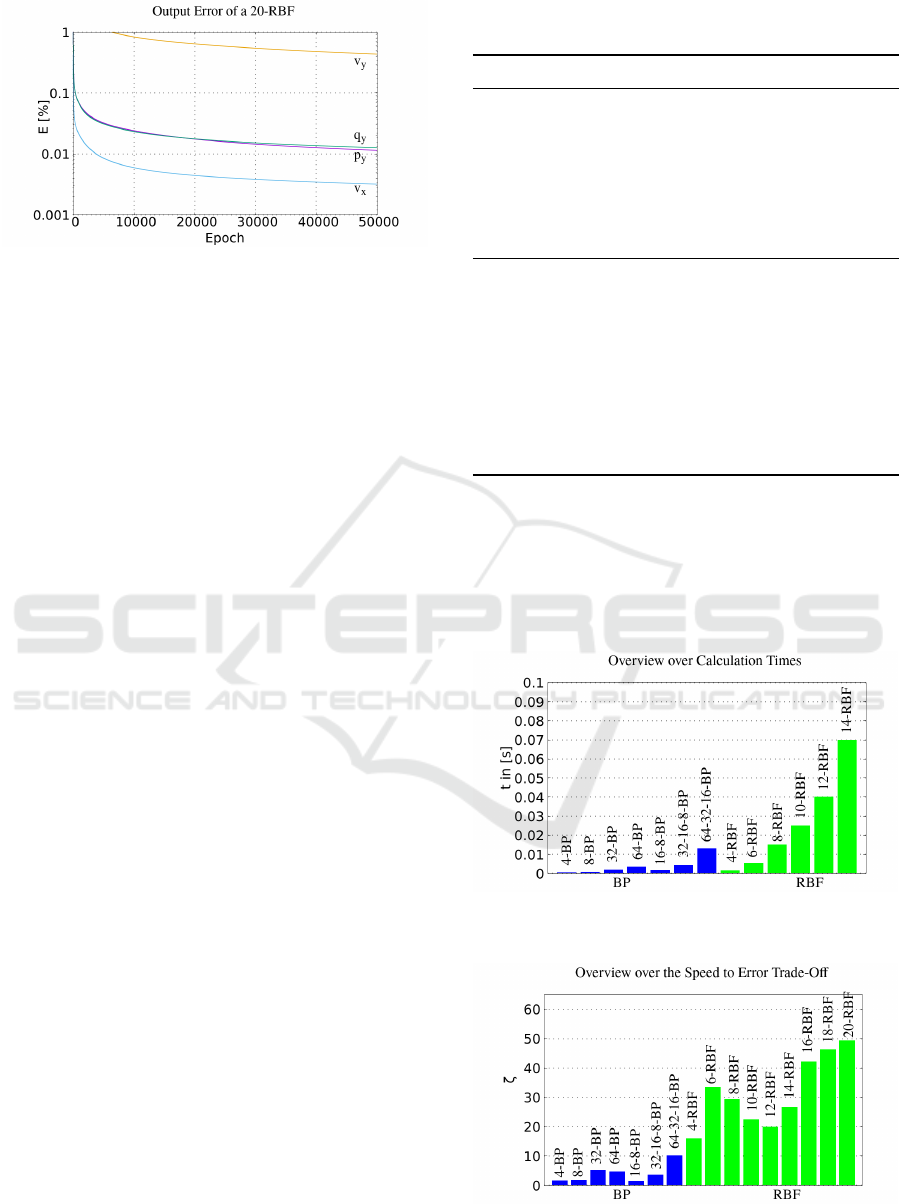
Figure 8: The resulting error of the radial basis function
with 20 neurons over the learning process.
Comparison of Errors: Both types of the dis-
cussed network architectures, were able to learn and
calculate the data as seen in Figs. 5 and 8. Remark-
able is that all networks required significantly more
time to learn the v
y
parameter compared to the other
three parameters. The reason for this is yet unclear, as
the parameters p
y
and q
y
depend on the same timing
inputs as v
y
.
Table 1 summarizes the final resulting errors of
the networks after 50 000 epochs. The results show
that the best error was achieved with the radial basis
function network with a total error of 0.218 %. The
best backpropagation network is the one containing
three hidden layers with h
1
= 64, h
2
= 32 and h
3
= 16
neurons resulting in an error of 0.72 %. The back-
propagation network with fewer layers and neurons
show a higher error rate. The maximum error has the
backpropagation network with four neurons of approx
3.2%.
Comparison of Calculation Time: As presented in
Table 2, the examined network architectures show a
significant difference in the calculation time. Figure 9
presents the time that the networks require to calcu-
late 1000 entries of the dataset. The amount of neu-
rons in the 4-BP and 4-RBF are the same and also
the calculation time is roughly the same. This is not
the case for the 8-BP and 8-RBF networks. Both
have the same count of neurons, but the difference
in calculation time is significant: t
8−BP
= 0.7[ms] to
t
8−RBF
= 12.8[ms]. The calculation time of the RBF
rises exponentially with the count of neurons.
Error to Speed Ratio ζ: In addition to the calcu-
lation times, Table 2 also presents the ζ-factor.. Fur-
ther, Fig. 10 gives an overview over the ζ-factors for
the different networks. The factor is not the same
for every network. The lower the value, the better
the calculation time to error ratio is. In general, the
backpropagation networks have a significant lower ζ-
Table 1: Summary of the percentual error of the BP and
RBF with different configurations after 50,000 epochs.
network p
yStart
p
yEnd
v
x
v
y
E
total
4-BP 2.83 3.06 3.20 3.93 3.28
8-BP 2.09 2.52 1.74 3.23 2.46
32-BP 1.97 2.54 1.39 4.17 2.72
64-BP 1.41 1.96 0.45 1.08 1.34
16-8-BP 0.65 1.45 0.42 0.71 0.90
32-16-8-BP 0.32 1.51 0.23 0.33 0.79
64-32-16-BP 0.17 1.52 0.15 0.24 0.78
4-RBF 3.08 3.48 2.74 20.8 10.7
6-RBF 0.59 0.79 0.43 12.5 6.32
8-RBF 0.15 0.20 0.08 4.57 2.29
10-RBF 0.05 0.07 0.02 1.74 0.87
12-RBF 0.02 0.03 0.004 0.94 0.47
14-RBF 0.02 0.02 0.005 0.77 0.38
16-RBF 0.01 0.02 0.004 0.71 0.36
18-RBF 0.01 0.01 0.004 0.60 0.28
20-RBF 0.01 0.01 0.0003 0.43 0.21
factor than the radial basis function networks. The
RBF show two sweet spots of the performance that
peak at the neuron counts of four and 12 neurons. By
contrast, the backpropagation networks show no real
sweet spots. The 16-8-BP shows the best performance
of the BP networks.
Figure 9: Speed comparison for different neural networks
for calculating 1000 entries of the dataset.
Figure 10: Comparison of the speed-to-error ratio ζ of the
networks. The lower the value the better the ratio.
SENSORNETS 2022 - 11th International Conference on Sensor Networks
102

Table 2: The table presents the required calculation times
of the networks to calculate 1000 entries of the dataset. In
addition, the total error and an error to calculation-time are
presented.
network t in [ms] E
total
E
total
∗ t
4-BP 0.5 3.28 1.6
8-BP 0.7 2.46 1.7
32-BP 1.9 2.72 5.1
64-BP 3.5 1.34 4.7
16-8-BP 1.7 0.90 1.5
32-16-8-BP 4.4 0.79 3.5
64-32-16-BP 13.1 0.78 10.2
4-RBF 1.5 10.72 16.0
6-RBF 5.3 6.32 33,5
8-RBF 12.8 2.29 29.3
10-RBF 25.7 0.87 22.4
12-RBF 42.1 0.47 19.9
14-RBF 70.1 0.38 26.6
16-RBF 117.4 0.36 42.1
18-RBF 165.3 0.28 46.2
20-RBF 226.4 0.21 49.3
6 DISCUSSION
This paper has presented a system that measures the
two-dimensional velocity of an object on the basis of
timestamps generated by light barriers. In compari-
son to the conventional approach, these light barriers
are set up not only in an orthogonal angle with re-
spect to the direction of movement, but also inclined
to it. When an object moves through these light bar-
riers, the system generates four timestamps which are
passed on to a neural network. The network retraces
both the path of the object and its two-dimensional
velocity.
In addition, multiple neural network architectures
were explored in order to investigate the effects of the
number of layers and neurons on the learning time and
formal precision as well as the execution time of the
networks. Therefore, the ζ-factor was introduced to
measure the speed-to-error ratio. The created datasets
were used to train and test these different architec-
tures.
Table 1 shows that the overall best performance
was achieved by the radial basis function network
with an error of 0.218 %. The lowest error of the back-
propagation networks was achieved by network which
consists of three hidden layers with the following neu-
ron count: h
1
= 64, h
2
= 32, and h
3
= 16. Although
the network had a lower average error than the others,
the result of a network with four neurons is sufficient
for an application such as curling.
On the one hand, the difference between the aver-
age errors of backpropagation network 4-BP and 64-
32-16-BP with 3.28 % versus 0.78 % have a low im-
pact on the resulting error of the system. On the other
hand, the reduced amount of neurons have a high im-
pact on the required computational resources of the
evaluation unit, e.g., the memory footprint of the pro-
gram and the calculation time for re-training. This
is shown by the ζ-factor: a larger network does not
decrease the error in the same amount as the calcu-
lation time rises. However, the network with four
neurons could be used on a smaller microcontroller,
e.g., ESP8266, whereas a larger network requires a
larger and more expensive hardware solution. The
best speed-to-error trade-off is achieved by a 16-8-
BP network. The same line of argumentation holds
to the radial basis function networks, where the best
trade-off is achieved with an 12-RBF. Therefore, for
the present application, the best network choice is
a backpropagation network with merely one hidden
layer with four neurons.
The results presented in this paper are generated
by simulations and without a practical validation. In
comparison to a physical application, the simulation
contained an abstraction of the objects in regard to
size and dimension. The simulated objects were com-
paratively smaller than curling stones which have a
diameter of 28.8 cm. Without re-training of the net-
work with real trajectories, the output of the network
is prone to error. In addition, the simulated trajecto-
ries of the objects have a constant velocity while mov-
ing through the light barriers. In a practical scenario,
friction effects would occur. However, these might
be neglectable due to the light barriers dimensions, at
least in the sport of curling.
As described in Section 4, the networks were
trained with a fixed learning rate, which results in
fluctuations of the errors as has been further addressed
in Section 5. Future work will be devoted to the im-
plementation of an adaptive learning rate to speed up
the training process, to reduce the fluctuation as well
as error plateaus and to reduce the resulting error. Fur-
thermore, future research will consider the extension
of the simulation with more light barriers to calculate
accelerations. The final step will consists in building
such a system in a real-world application.
7 CONCLUSION
In summary, this paper closes with the following con-
clusions: The system of Surface Light Barriers is able
to calculate the two-dimensional speed of an object
through a smart positioning of multiple light barriers.
Surface Light Barriers
103

Both, backpropagation neural networks and radial ba-
sis function networks are able to learn the model of
the Surface Light Barriers. A neural network with
four neurons is able to learn the model with an accept-
able error rate of E < 4%, which is sufficient for sport
application. These small neural networks can be used
on microcontrollers with low-power hardware. For
applications which require a higher accuracy, more
complex neural networks with multiple layers are able
to achieve an error of E < 0.3%.
ACKNOWLEDGEMENT
The authors gratefully thank the German Curling As-
sociation (Deutscher Curling Verband) for providing
this engineering task.
REFERENCES
Phansalkar, V. and Sastry, P. (1994). Analysis of the back-
propagation algorithm with momentum. IEEE Trans-
actions on Neural Networks, 5(3):505–506.
Tao, K. (1993). A closer look at the radial basis function
(rbf) networks. In Proceedings of 27th Asilomar Con-
ference on Signals, Systems and Computers, pages
401–405 vol.1.
Wythoff, B. J. (1993). Backpropagation neural networks:
A tutorial. Chemometrics and Intelligent Laboratory
Systems, 18(2):115–155.
A VECTOR CALCULATIONS
In the following, each light barrier is seen as a vector con-
sisting of a starting point P
i
= (p
ix
, p
iy
)
T
and a direction of
the beam of light.
⃗
B
i
= (b
ix
,b
iy
)
T
.
LB
i
= P
i
+ s
i
⃗
B
i
(11)
The object O moves through the light barriers with a
starting point and a constant speed vector
⃗
V = (v
x
,v
y
)
T
:
O = P
O
+t
⃗
V
O
(12)
The entrance point of the object in the section of mea-
surement is called P
start
= (0,y
start
)
T
. The point of leaving
is called P
end
= (p
4x
,y
end
)
T
. To the differential timings,
as stated in Eq. 1, can be added the following differential
timing:
∆t
23
= t
3
−t
2
(13)
The final formulars for the calculations are:
v
x
=
p
x4
− p
x1
∆t
4
(14)
v
y
=
(∆t
23
v
x
− p
3x
)b
3y
b
3x
∆t
23
(15)
y
start
= p
2y
+

∆t
4
v
x
−
p
2x
b
2x

b
2y
− ∆t
4
v
y
(16)
y
end
= y
start
+ v
y
∆t
4
(17)
SENSORNETS 2022 - 11th International Conference on Sensor Networks
104