
Comparison of Two Different Radar Concepts for Pedestrian
Protection on Bus Stops
E. Streck
1
, R. Herschel
2
, P. Wallrath
2
, M. Sunderam
3
and G. Elger
3
1
Faculty Electrical Engineering and Computer Science, Technische Hochschule Ingolstadt,
Esplanade 10, Ingolstadt, Germany
2
Fraunhofer Institute for High Frequency Physics and Radar Techniques FHR, Wachtberg, Germany
3
Fraunhofer Institut für Verkehrs- und Infrastruktursysteme IVI, Ingolstadt, Germany
{Mohan.Sunderam, Gordon.Elger}@ivi.fraunhofer.de.
Keywords: Sensor Data Fusion, Radar Sensor, Multiple-Sensor Systems. Machine Learning.
Abstract: This paper presents the joint work from the “HORIS” project, with a focus on pedestrian detection at bus-
stops by radar sensors mounted in the infrastructure to support future autonomous driving and protecting
pedestrians in critical situations. Two sensor systems are investigated and evaluated. The first based on single
radar sensor phase-sensitive raw data analysis and the second based on sensor data fusion of cluster data with
two radar sensors using neural networks to predict the position of pedestrians.
1 INTRODUCTION
Nowadays, in automotive and infrastructure radar
sensors, LiDAR sensors and camera-based solutions
are used to increase the safety of the traffic and enable
smart city solutions (Kumar, 2021). To increase the
security level especially for vulnerable road users
(VRU’s) like pedestrians or cyclists, sensors are used
in driver assistance systems in the car and in future
also in infrastructural applications, e.g., automatic
traffic light management systems. Every sensor has
its advantages and drawbacks. In contrast to camera,
whose strength lies in the classification, the strengths
of the radar sensor are in the accuracy of the distance
measurement and the extraction of the velocity
directly from the utilization of the Doppler Effect. On
the other hand, the strength of the LiDAR sensor is in
between, as it can be used as output for a good
classification due to its dense point cloud and it can
provide a very precise spatial resolution of the point
cloud (Yeong, 2021). Nevertheless, the LiDAR
sensor is currently relatively expensive compared to
cameras and radar sensors. Another advantages of
radar sensors are that they have high reliability in bad
weather conditions (e.g., rain, fog, snow, etc.) as well
as in night detection. In addition, radar data are
uncritical regarding privacy: No sensitive personal
data are measured, i.e., the data are completely
anonymous in contrast to camera data. For this
reason, radar sensors are an integral part of a wide
variety of applications and therefore the focus in this
paper is on the pedestrian detection using radar
sensors in the infrastructure, but the presented use
case could also be carried out by Camera or LiDAR.
In previous related works on pedestrian detection the
localization and classification are carried out by some
state-of-the-art methods like Micro-Doppler (Lam,
2016), methods based on doppler spectrum and range
profiles (Rohling, 2010), utilization of the range
azimuth map to estimate the dimensions of an object
(Toker, 2020), etc. In this paper, two different
approaches using the variance by utilizing the raw
data and using neural networks by utilizing the high-
level data, with different sensor systems for detecting
pedestrians on bus-stops with high accuracy in a joint
Fraunhofer project “HORIS” will be presented. First,
the project and the used sensor systems will be
described. Next, the two sensor systems are discussed
in more detail and the working principle of the
algorithms is presented. Finally, the performance of
the detection capability of the two systems is
evaluated and compared.
2 PROJECT PRESENTATION
HORIS
At this point the project HORIS is presented in which
the results for this paper were generated. Project
Streck, E., Herschel, R., Wallrath, P., Sunderam, M. and Elger, G.
Comparison of Two Different Radar Concepts for Pedestrian Protection on Bus Stops.
DOI: 10.5220/0010777100003118
In Proceedings of the 11th International Conference on Sensor Networks (SENSORNETS 2022), pages 89-96
ISBN: 978-989-758-551-7; ISSN: 2184-4380
Copyright
c
2022 by SCITEPRESS – Science and Technology Publications, Lda. All rights reserved
89
HORIS stands for "High Resolution Radar Sensors in
the Infrastructure", which is a joint Fraunhofer project
(sponsored by CCIT-COMMs) of the following
institutes:
Fraunhofer FHR,
Fraunhofer IIS,
Fraunhofer IVI.
The applicational focus on this paper is on a bus-
stop, where the sensors are mounted in a fixed
distance to each other on the opposite side of the road
and observed will be a crowd of people. A trigger
event is provided if a person starts crossing the street
and enters the danger zone e.g., to catch the bus on
the opposite side of the road. In this scenario, the
objects are roughly in 5-15m distance away from the
sensor system. Once a person entering the danger
zone, a message via Car2X communication can be
sent to alert the surrounding vehicles. However, the
paper focuses on the radar technology, whereas the
communication via Car2X is not discussed any
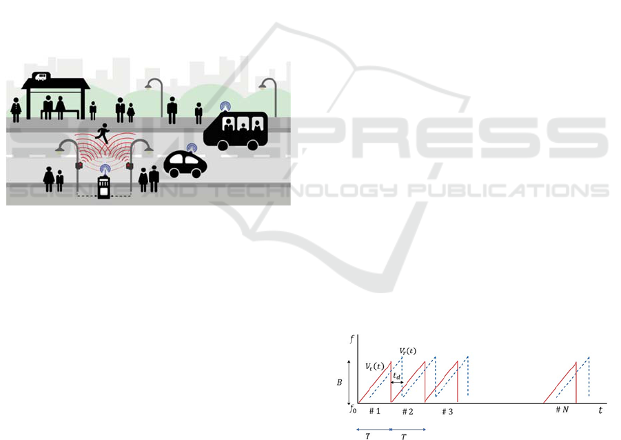
further. A schematic representation of the use case
can be seen in Figure 1.
Figure 1: Radar sensors, locating on the opposite side of the
road, detects a pedestrian, which is leaving the static group
while crossing the street. Car2X message is sent out from
central unit to warn the surrounding traffic.
Two different sensor approaches, which operate on
80 GHz radar technology were used. The first
approach uses a radar sensor based on the TI chipset,
which can quickly detect the smallest movements
with a very high frame rate with the help of phase-
sensitive raw data analysis. Especially the
investigation of the correlation degree of the
movement patterns of a crowd of people with the full
utilization of the raw data is done and will be
discussed in more detail in section 4. The second
approach uses two commercial radar sensors from the
automotive industry built into the infrastructure,
which will be fused based on neural networks (NNs).
For the second approach, it will be investigated,
whether the high-level cluster data output by the
sensor results in an improvement of the detection
accuracy with two radar sensors in contrast to one
sensor that works based on a state-of-the-art tracking
algorithm based on "density-based spatial clustering
of applications with noise" (DBSCAN) (Dingsheng
Deng, 2020). The NN approach will be discussed in
more detail in section 5. The reason of using two
instead of a single radar sensor with NNs is that such
conditions were defined in this 6-month project
before and the results of one sensor will be presented
in a separate work. The sensors are operated with
Robot Operating System (ROS), since this
framework is well suited for data fusion, real time
processing and visualization. The data collection and
data acquisition for the development of the signal
processing, the tracking, and the classification, as
well as for the training, validation and test of the
neural networks is done by an optical-based
localization system with an accuracy of 1mm and
using PTP software synchronization with an accuracy
of ∆t ≤ 0.5ms provided by Fraunhofer IIS.
3 RADAR TECHNOLOGY AND
DATA PROCESSING
Since the “Frequency Modulated Continuous Wave”
FMCW radar (Skolnik, 1990) is the most used
scheme in automotive today, the HORIS project also
uses radar sensors, based on the FMCW technology,
with which it is possible to achieve good spatial
resolution with a comparatively lower transmission
power in comparison to a pulsed radar sensor. The
following section briefly explains how the FMCW
radar works (Engels, 2021). The frequency bands for
the used sensors are in the range of 77-81 GHz, which
defines one of the most important allowed frequency
bands for automotive. The FMCW radar sweeps wide
radar frequency (RF) bandwidth (in GHz), while
keeping the intermediate frequency (IF) bandwidth
small (in MHz) and this working principle is shown
in Figure 2.
Figure 2: The radar sweeps with a defined bandwidth B for
a chirp duration T on the carrier frequency 𝑓
, which is in
the range of 77-81 GHz. Multiple chirps are generated with
this sawtooth sweep principle and send out by a frame
containing the total N chirps.
A simple schematic block diagram of such a FMCW
radar can be seen in Figure 3.
SENSORNETS 2022 - 11th International Conference on Sensor Networks
90
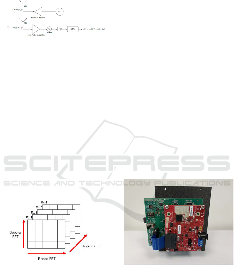
Figure 3: The Tx antenna sends the radio wave out, which
will be reflected by a static or moving object and the
delayed signal will be received back by the Rx antenna. The
frequency mixer subtracts the frequencies of the received
signal from the generated signal, which results in the
intermediate frequency (IF) of each transmitter & receiver
pair.
Since the IF is proportional to the radial distance
between radar sensor and object, the distance can be
calculated using the first dimension FFT of the
received IF signal. For moving objects, the velocity
can be calculated using the phase change across
multiple chirps and therefore a second dimension FFT
is performed to determine the phase change and thus
the velocity of objects in form of a e.g., range velocity
image. For the angle estimation of detected objects,
the received signal is registered by multiple antennas.
The distances of the reflected wave to the receiver
antennas are now different with respect to the angle
of arrival for each Rx. This results in a phase change,
which can be estimated using the third dimension
FFT and finally the angle of arrival can be extracted.
Since the 1D FFT processing is done inline in the
active transmission time of the chirps, the 2D & 3D
FFT is processed “offline” in the inter-frame time.
This information output is the so-called radar cube
and is shown in Figure 4.
Figure 4: The columns for the FMCW radar cube are filled
with range, the rows with doppler velocity and the depth
with the angle information (Sturm, 2016).
After this data has been processed with the help of the
so-called constant false alarm rate (CFAR) algorithm
(Finn and Johnson, 1968), which calculates an
adaptive threshold value due to the estimated noise
floor to reduce the number of false detections, clutter
and noise, the remaining data is also referred to as the
so-called point cloud data. The sensor approach,
presented in section 4, is based on 3D voxels in
Cartesian coordinates, whereas the sensor system
presented in section 5 is based on processed point
cloud data, the so-called “cluster data”, using similar
algorithms to DBSCAN. The radar sensor presented
there has a limited data transfer rate, since it is
operating with CANBUS instead of using a high
speed ethernet interface. Since the bandwidth of the
cluster data is very reduced (few MB/min) in
comparison to the whole radar cube (few GB/min),
both sensor systems, which are based on phase
sensitive raw data analysis and cluster data analysis
using machine learning (ML) techniques, will be
presented in the upcoming sections.
4 FHR RADAR SENSOR AND IT’S
ALGORITHM
4.1 The Sensor
For the measurements, an integrated MIMO radar
sensor from TI was used. This includes 3 transmitters
and 4 receivers. Only 2 transmitters were used
resulting in 8 antenna combinations forming a single
line in azimuth. This allows an azimuth resolution of
15 degrees. To get access to the raw data the
AWR2243 BOOST board from TI was combined
with a DCA1000 as shown in Figure 5.
Figure 5: MIMO radar module used for people detection.
The radar supports 4 GHz bandwidth. However only
380 MHz bandwidth were used to be able to support
a framerate of 2 kHz to monitor people with a high
frequency to detect small movements. The raw data
was received over Ethernet online processed on the
PC and the result published using a ROS interface.
Comparison of Two Different Radar Concepts for Pedestrian Protection on Bus Stops
91
4.2 Signal Processing
The signal processing included two major steps. First,
the scene was captured with people standing at a
defined distance from the radar. In that initialization
step it was crucial to determine the position of the
person in the scene. For test measurements people
were standing 5m from the radar sensor.
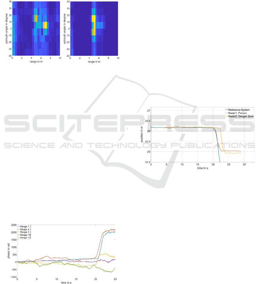
Figure 6: Range-Azimuth map of the measured scene based
on the reflected power (left) and the variance of the
reflection over time (right).
As one can clearly see in Figure 6 it is hard to see the
persons in the scene if only the magnitude of the
reflectivity is considered. Static reflections from the
bus stop are dominating the image. That significantly
changes if the variance over time is taken over 5s.
Since variance calculation includes the subtraction of
the mean value, static targets are well suppressed. As
shown on the right, all three persons can be seen
standing beside each other. That allowed to monitor
the signal phase at the voxels of relevance. However,
the movement of each person also lead to a significant
variance at further range bins, caused by moving
shadows. Therefore, the phase of various voxels was
monitored. From that range-azimuth map, it can be
hard to distinguish individual persons. However, the
movement within each voxel can be taken as an
alternative feature to identify different individually
moving objects. This is currently a subject under
investigation.
Figure 7: Temporal phase development for range bins 7-11
for azimuth:9. Movement of pedestrian can be extracted by
range bins 7 and 8.
Figure 7 shows the phase of several selected voxels.
To only select one person, only a single azimuth bin
was chosen. The two closest range bins appear to be
the best monitor for the movement of the person.
Before starting to walk fluctuations can be seen
caused by gesticulations or moving at the same
position. Even vital parameters such as pulse and
respiration can be extracted if the phase fluctuation is
filtered accordingly (Rudrappa, 2020). Signals from
range bins behind the person are far weaker, so that
their phase fluctuation is dominated by receiver noise.
However, range bin 8 shows the movement of the
person with smaller latency. Since the person is first
moving forward with its upper body before moving
the leg (usually being in front) that is not unexpected.
A fixed threshold was defined to cause an interrupt
for all channels. Since the monitor of all voxels was
combined by a logical AND the first movement
caused the alarm, it did not make a difference where
the first movement occurred.
After the first alarm, a second alarm was defined
at a predefined range bin. In that case, no detection
was required. The same approach for phase detection
was used.
Figure 8: Phase tracking at position of the monitored person
(red) and at the range bin defined to be critical (yellow) in
comparison to the position of the person measured with an
optical marker (blue).
In Figure 8 the red curve shows the movement
detected on the voxel where the person was detected
during the initialization phase. It shows a very strong
correlation to the movement detected by an optical
Qualisys system. Differences are likely to be caused
by the different parts of the body monitored with
optical and radar system, since the marker was fixed
on the helmet of the person. The correlation ends as
soon as the person left the voxel under test. After
entering the second range bin which defines the
transition to a critical area the yellow curve follows
the movement of the person. Now, the second alarm
is caused before the person leaves the monitored
voxel. For a constant monitoring the position of the
person must be tracked so that always the correct
SENSORNETS 2022 - 11th International Conference on Sensor Networks
92

voxel is chosen. This has not been required in that
scenario but was also realized to measure the vital
parameters of walking persons in as separate work
(Rudrappa, 2020).
5 TWO RADAR SENSOR ML
APPROACH
In this section the prediction of the localization of
pedestrians with two commercial Conti ARS408-21
automotive radar sensors, operating on raw untracked
detections, using a neural network (NN) based on
high-level cluster data is presented. First, the data
processing for the training is discussed. Later the NN
structure is presented, and the training results are
discussed. Finally, a comparison of the localization
capability of the two-radar sensor ML approach with
respect to one single radar sensor operating with a
state-of-the-art tracking algorithm, like the Hungarian
(Kuhn, 2012) algorithm modified with a clustering
DBSCAN algorithm is presented.
5.1 Data Processing
To train a NN model, it is necessary to use prepared
data in an appropriate format as input to speed up the
training and save computational resources. The frame
rate of the radar sensors is approx. 14 fps and the
cluster data are from the following shape: position
coordinates, radial velocity, and Radar Cross Section
(RCS). Since the internal software on the radar
prioritize moving detections before static ones and
therefore several static clusters will be filtered out, the
approach presented here covers only dynamic objects,
since for the application it is necessary to detect
pedestrians entering the danger zone. In (Streck,
2021) a possible solution also for static objects is
presented. For a general use case it is reasonable to
use a radar sensor, which has also a good static object
detection. To obtain a proper data format for the
training process first, a coordinate transformation for
both radar sensors in a common coordinate frame
(chosen as center of mass of both radar sensors) is
made. Second, since the update rates for both sensors
are not exactly coinciding a time synchronization for
both sensors was performed, whereas every frame of
sensor A should be assigned to the time nearest frame
of sensor B. Because both radar sensors are seeing the
same scene from different perspectives with a
different number of reflections, it is sometimes
necessary to throw out one frame of sensor A or
sensor B to achieve a proper assignment of frames.
With this simple time synchronization method, the
maximum delay between two frames from both radars
can be estimated to 35.7ms, which leads to an
uncertainty of around 6cm. With this software
synchronization algorithm, the results are acceptable
and could be further improved using a hardware
synchronization. Since the focus lies on pedestrian
detection it is reasonable to filter those cluster out,
which contributes to noise. For the training those
cluster of non-characteristic RCS as for pedestrians
are omitted. In general, it was found out by
experimental measurements that the range of the RCS
to detect pedestrians is between [-30,5] dBm². Using
this method, the total amount of clusters could be
reduced by roughly 40%.
5.2 Neural Network Structure and
Training
As mentioned above, the model respects only
dynamic objects, since static ones with a lower RCS
(especially for pedestrians, which are enveloped by
the bus-stop) cannot be detected in every frame
constantly. This lack of detection causes a problem
for the training. The input for the training is extracted
from the whole data set, which includes 160k samples
(static & dynamic objects) and is of the size of 23k
effective sample frames. Additional data was also
created by mirroring the data with respect to the x-
axis (radar coordinate frame). In the following,
TensorFlow 2.1 (Abadi, 2015) and Keras (Chollet,
2015) were used as the python library for the training
and evaluation of the NNs. Since the trained
cooperative sensor system will be operating in the
infrastructure mounted at a fixed place, without loss
of generality, a region of interest (ROI) was chosen
as a surface, spanned by 15m x 18m in the lateral and
longitudinal direction, respectively, which starts 1m
from the common sensor system coordinate frame.
The shape of the input and output data for the NN is
chosen as a pixel representation of the ROI, in which
the algorithm should perform for a variable number
of detected pedestrians. For simplicity the ROI is
divided into three different pixel size models. These
different models, together with the resolution for each
pixel cell, as well as its probability of the prediction
of a pedestrian using the test-set evaluation is shown
in table 1, whereas the NN structure achieving these
probabilities will be discussed later in this sub-
section. One can also see that the probabilities are
smaller the larger the pixel model gets, which is
reasonable, since with greater pixel models the
prediction of the exact pixel localization of a
pedestrian gets much harder.
Comparison of Two Different Radar Concepts for Pedestrian Protection on Bus Stops
93
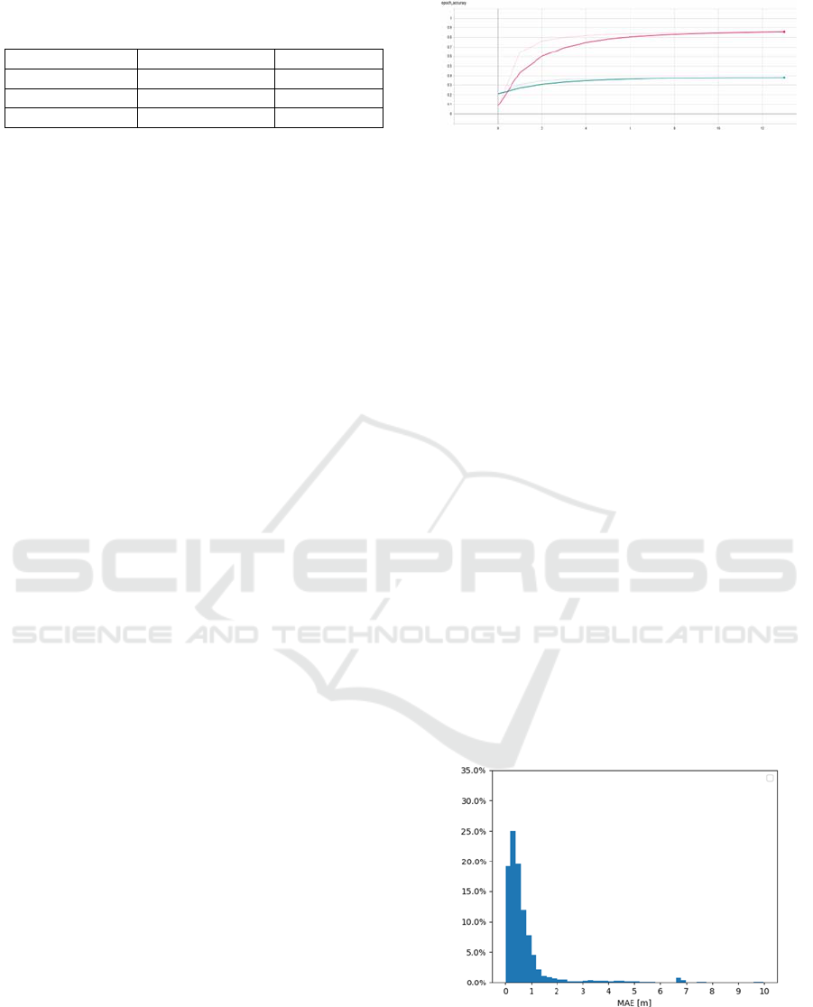
Table 1: Overview of test probabilities of corresponding
pixel resolutions.
Model Pixel Size [m] Probabilit
y
5 x 6 3.0 0.90
15 x 18 1.0 0.73
75 x 90 0.2 0.36
The whole data used for the training is separated in
0.44, 0.22 and 0.33 for train-, validation- and test-set,
respectively. The features of the input vector for the
NN are defined as the frequency of occupancy of the
clusters for each pixel cell, the radial velocity of the
pixel cell and their corresponding RCS value. These
three features are representing a pixel, where its
values are divided into the color-coded range of
[0,255]. The output array for localization can be
represented as
y
⃗
𝑙
,
𝑙
,
⋯𝑙
,
𝑙
,
𝑙
,
⋯𝑙
,
⋮⋮⋱⋮
𝑙
,
𝑙
,
⋯𝑙
,
,
(1)
where 𝑙
,
is the pixel occupancy for sample i and
pixel j, counting from the left upper corner of the
pixel representation of the ROI, which is
𝑙
,
1 ,𝑖𝑓 𝑝𝑖𝑥𝑒𝑙
𝑗
𝑖𝑠 𝑜𝑐𝑐𝑢𝑝𝑖𝑒𝑑
0 ,𝑒𝑙𝑠𝑒.
(2)
For further discussion of the architecture and the
training the (90x75)-model is selected, which defines
the size of the input image as total 6750 pixels plus
three-color channels for the input parameter, since
this representation is the most accurate one for the
presented use case. For this purpose, a DNN (Huang,
2016) architecture was used. The reason why for the
training a DNN instead a CNN was chosen is, since
the density of the cluster data is much lower than that
of a point cloud, the dynamic objects doesn’t show
such good shapes and features which could be
detected nicely by the CNN, therefore a simple fully
connected NN with more training parameters was
chosen. This model takes as input a picture of size
(90x75) with three color-channels and flatten these
inputs to get an array with the length of 20250. This
is the input for the next dense layer of size 6750,
which represents the total number of all pixels, since
the output in the end predicts the occupied pixels in
the ROI. After the dense layer a “tanh” (Hyperbolic
Tangent) (Nwankpa, 2018) activation function was
applied because it can integrate non-linearities into
the model much easier than the “relu” activation
function in comparison. Due to the enormously large
input for the last dense layer, the total number of
parameters increases up to 136,694,250.
Figure 9: Training (red) and validation (green) accuracy of
the trained dynamic model with following settings:
RMSprop as optimizer, batch normalization, batch size of
256 and learning rate of 0.000774 found using the
ReduceLROnPlateau.
Figure 9 shows the training performance, where a
modified MSE loss function was used, which
regulates the predictions based on the weighting for
neighbor predictions as a kind of penalty mechanism.
This controls somehow the maximum number of
predictions. As already stated in table 1, the final test
accuracy for the corresponding trainings accuracy of
0.87, is 0.36. Unfortunately, one can clearly see, that
the system was learned due to the clear signs of
overfitting. This problem will be overcome when
larger amount of data, as well as more general data
for the training will be measured. Also, a possible
improvement of the model might be the extension of
the input space. Nevertheless, this model is chosen for
the final evaluation of the results.
5.3 Localization Results
At this point the localization capability of the NN
approach in comparison with the single-radar sensor
system, based on DBSCAN algorithm, mentioned at
the beginning of this section, will be presented. For
the bus-stop use case, the mean absolute error was
used to analyse the localization accuracy. The
Figure 10: Evaluation of the mean absolute error of the
localization for the single radar system, using tracking
algorithm. In total 40796 frames were evaluated, and the
histogram was normalized due to this value.
SENSORNETS 2022 - 11th International Conference on Sensor Networks
94
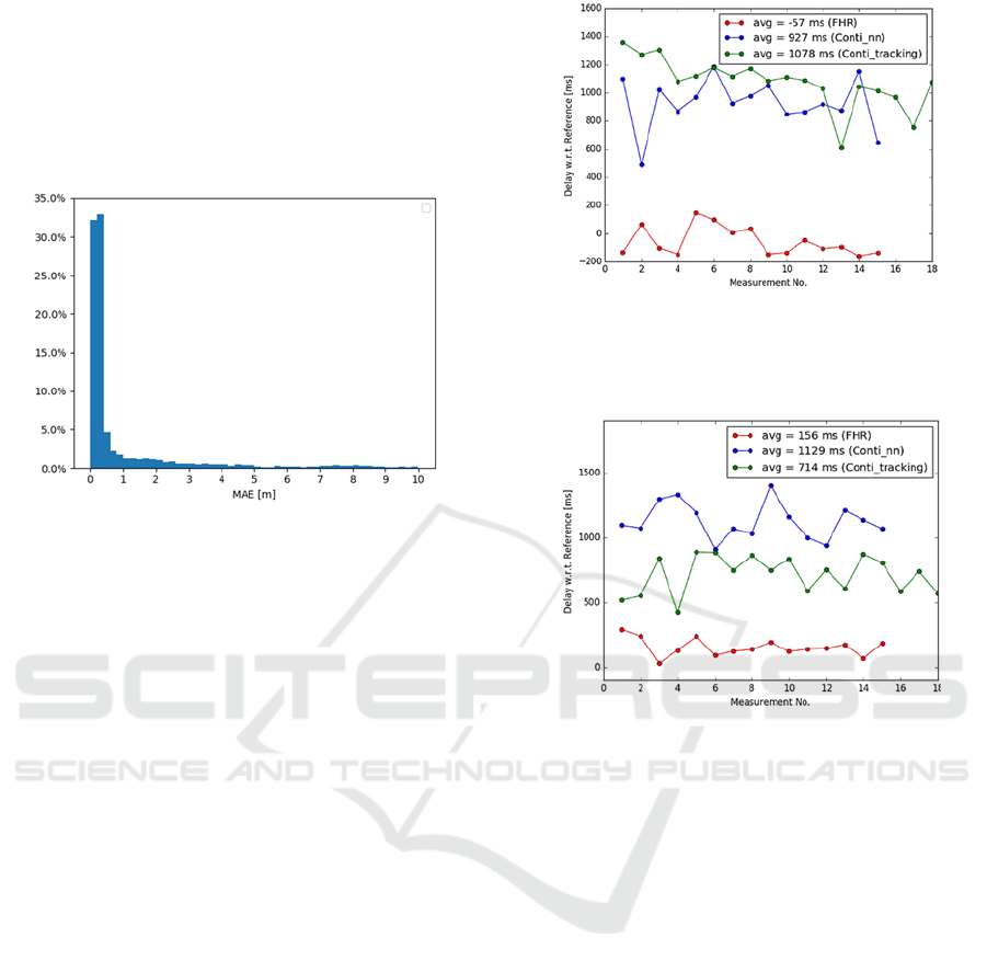
evaluation of the single-radar sensor approach is
shown in Figure 10, whereas one can see, that approx.
44% of the total amount of predictions are within
0.4m accuracy.
The evaluation of the two radar NN approach is
shown in Figure 11 and one can see, that 66% of the
predictions are within 0.4m accuracy.
Figure 11: Evaluation of the mean absolute error of the
localization for the NN approach of total 7666 frames, and
the histogram was normalized due to this value.
Since the resolution of the used radar sensors is
anyway 0.4m, this value is used as a reference. In both
histograms one can also see that outliers for larger
deviations of 0.4m can occur. In Figure 10 these false
positives are the detections of incorrect objects by the
used tracking algorithm, while noise is likely to be
detected as an object that clearly doesn’t match the
reference data and therefore represents false
detections for the single radar system. In Figure 11
these deviations come from the forecast of the NN,
which sometimes predicts several ghost targets, since
the total number of pedestrians in the scene is
unknown for the NN.
6 COMPARISON & OUTLOOK
For the time evaluation of both presented sensor
models in section 4 and 5, a set of photoelectric
barriers was placed approx. 30cm in front of the
pedestrian, which defines start of movement into
danger zone and one in front of the entrance to the
danger zone. Figure 12 and 13 show the comparison
of the detection time delay of both sensor systems
w.r.t. the photoelectric barriers.
Figure 12: Comparison of the detection delays of the phase-
sensitive evaluation (red), NN approach (blue) and a single
sensor tracking algorithm (green) for the start of the motion
of a pedestrian.
Figure 13: Comparison of the detection delays of the phase-
sensitive evaluation (red), NN approach (blue) and a single
sensor tracking algorithm (green) for the entrance into the
danger zone.
In both measurements one can see that the
performance of the phase sensitive solution using raw
data performs around 1s better than the NN approach
with two commercial radar sensors, operating on
cluster data. The negative value in Figure 12 of the
FHR detection comes from the fact that for the
demonstration the light barrier was placed a bit too far
from the pedestrian which initialized the movement.
For the comparison also the time performance of the
single-radar solution is plotted, which for the entrance
into the danger zone performs around 300ms faster
and for the detection of the motion around 150ms
delayed in comparison to the NN solution. This is due
to the fact, that the single-radar approach works with
a tracking algorithm based on establishing the track
by comparing frames of the past. So, this system
needs an initialization time which is around 450ms to
track the pedestrian. To increase the performance of
the NN approach and to overcome the overfitting
problem and to achieve a better prediction accuracy,
the net could be retrained using more training data.
Also, for reduction of false positives more
Comparison of Two Different Radar Concepts for Pedestrian Protection on Bus Stops
95

generalized data should be collected, as well as the
setup parameters (e.g., angles and position of the
sensors with respect to each other) should be
calibrated better. Nevertheless, the NN approach
looks promising and should be further investigated
because even with the actual simple overfitting
model, location performance could be substantially
improved as opposed to a single radar approach.
REFERENCES
K. K. kumar, E. Ramaraj and D. N. V. S. L. S. Indira, "Data
Fusion Method and Internet of Things (IoT) for Smart
City Application," 2021 Third International Conference
on Intelligent Communication Technologies and Virtual
Mobile Networks (ICICV), 2021, pp. 284-289, doi:
10.1109/ICICV50876.2021.9388532.
Yeong, De J., Gustavo Velasco-Hernandez, John Barry, and
Joseph Walsh. 2021. "Sensor and Sensor Fusion
Technology in Autonomous Vehicles:
A Review" Sensors 21, no. 6: 2140.
https://doi.org/10.3390/s21062140.
O. H. Y. Lam, R. Kulke, M. Hagelen and G. Möllenbeck,
"Classification of moving targets using mirco-Doppler
radar," 2016 17th International Radar Symposium
(IRS), 2016, pp. 1-6, doi: 10.1109/IRS.2016.7497317.
H. Rohling, S. Heuel and H. Ritter, "Pedestrian detection
procedure integrated into an 24 GHz automotive radar,"
2010 IEEE Radar Conference, 2010, pp. 1229-1232,
doi: 10.1109/RADAR.2010.5494432.
O. Toker and S. Alsweiss, "mmWave Radar Based
Approach for Pedestrian Identification in Autonomous
Vehicles," 2020 SoutheastCon, 2020, pp. 1-2, doi:
10.1109/SoutheastCon44009.2020.9249704.
Dingsheng Deng, “DBSCAN Clustering Algorithm Based
on Density,” 7th International Forum on Electrical
Engineering and Automation (IFEEA), 2020, pp. 949-
953, DOI: 10.1109/IFEEA51475.2020.00199.
M. I. Skolnik, Radar Handbook. Second ed, The McGraw-
Hill Co., 1990.
F. Engels, P. Heidenreich, M. Wintermantel, L. Stäcker, M.
Al Kadi and A. M. Zoubir, "Automotive Radar Signal
Processing: Research Directions and Practical
Challenges," in IEEE Journal of Selected Topics in
Signal Processing, vol. 15, no. 4, pp. 865-878, June
2021, doi: 10.1109/JSTSP.2021.3063666.
C. Sturm, G. Li, Gerd-Heinrichs, Urs Lubbert, “79 GHz
wideband fast chirp automotive radar sensors with agile
bandwidth“, IEEE MTT-S International Conference on
Microwaves for Intelligent Mobility (ICMIM), 2016,
doi:10.1109/ICMIM.2016.7533913.
H. M. Finn and R. S. Johnson, “Adaptive detection mode
with threshold control as a function of spacially
sampled clutter-level estimates;” RCA Rev., vol. 29,
pp. 141-464, September 1968.
M. T. Rudrappa, R. Herschel and P. Knott, "Distinguishing
living and non living subjects in a scene based on vital
parameter estimation," 2020 17th European Radar
Conference (EuRAD), 2021, pp. 53-56, doi:
10.1109/EuRAD48048.2021.00025.
Kuhn, H.. (2012). The Hungarian Method for the
Assignment Problem. Naval Research Logistic
Quarterly. 2.
E. Streck, P. Schmok, K.Schneider, H.Erdogan and G.
Elger, "Safeguarding future autonomous traffic by
infrastructure based on multi radar sensor
systems," FISITA 2021 World Congress, 2021, doi:
10.46720/F2021-ACM-121.
Abadi et al. 2015. TensorFlow: Large-Scale Machine
Learning on Heterogeneous Systems. (2015).
http://tensorflow.org/ Software available from
tensorflow.org.
François Chollet et al. 2015. Keras.
https://github.com/keras-team/keras. (2015).
Gao Huang, Zhuang Liu, Laurens van der Maaten, Kilian
Q. Weinberger, “Densely Connected Convolutional
Networks,” arXiv:1608.06993 (2016).
Chigozie Enyinna Nwankpa, Winifred Ijomah, Anthony
Gachagan, and Stephen Marshall, “Activation
Functions: Comparison of Trends in Practice and
Research for Deep Learning,” arXiv:1811.03378v1
(2018).
K. Ramasubramanian, B. Ginsburg, “Highly integrated
77GHz FMCW Radar front-end: Key features for
emerging ADAS applications”, 2017, Texas
Instruments.
SENSORNETS 2022 - 11th International Conference on Sensor Networks
96
