
What Matters for Out-of-Distribution Detectors using Pre-trained CNN?
Dong-Hee Kim
a
, Jaeyoon Lee
b
and Ki-Seok Chung
c
Department of Electronic Engineering, Hanyang University, 222 Wangsimni-ro, Seoul, Korea
Keywords:
Out-of-Distribution Detection, Convolutional Neural Network.
Abstract:
In many real-world applications, a trained neural network classifier may have inputs that do not belong to any
classes of the dataset used for training. Such inputs are called out-of-distribution (OOD) inputs. Obviously,
OOD samples may cause the classifier to perform unreliably and inaccurately. Therefore, it is important
to have the capability of distinguishing the OOD inputs from the in-distribution (ID) data. To improve the
detection capability, quite a few methods using pre-trained convolutional neural networks(CNNs) with OOD
samples have been proposed. Even though these methods show good performance in various applications, the
OOD detection capabilities may vary depending on the implementation details and the methodology how to
apply a set of detection methods. Thus, it is very important to choose both a good set of solutions and the
methodology how to apply the set of solutions to maximize the effectiveness. In this paper, we carry out an
extensive set of experiments to discuss various factors that may affect the OOD detection performance. Four
different OOD detectors are tested with various implementation settings to find the configuration to achieve
practically solid results.
1 INTRODUCTION
Since Hendrycks and Gimpel (Hendrycks and Gim-
pel, 2017) proposed a scheme for detecting out-of-
distribution (OOD) samples, various deep learning
methods have been suggested for detecting OOD
samples. Thanks to the development, the reliability
of the neural network classifier is improved. For in-
stance, Oberdiek et al(Oberdiek et al., 2020) proposed
an OOD detection method to solve a semantic seg-
mentation task for a driver-centric view segmentation
dataset, and Pacheco et al(Pacheco et al., 2020) pro-
posed a method to pick out images that are not suit-
able for skin cancer classifiers.
Among many OOD detectors, detectors based
on pre-trained convolutional neural networks (CNNs)
such as ODIN (Liang et al., 2018), Mahalanobis (Lee
et al., 2018b), and Gram (Sastry and Oore, 2020) have
gained lots of attention. These methods have the ad-
vantages that the network model does not have to be
re-trained. Namely, they do not require the full train-
ing dataset to conduct the end-to-end backpropaga-
tion. Furthermore, the pre-trained CNN-based detec-
tors can maintain the in-distribution (ID) classifica-
a
https://orcid.org/0000-0003-4787-8016
b
https://orcid.org/0000-0003-1350-0357
c
https://orcid.org/0000-0002-2908-8443
tion accuracy. It is a considerable advantage because
other previous works suffered from classification ac-
curacy degradation (Lee et al., 2018a; Hendrycks
et al., 2019a; Yu and Aizawa, 2019; Hsu et al., 2020).
Due to these merits, the pre-trained detectors are
widely adopted in practical applications. Therefore,
we will focus on the detectors based on pre-training
in this paper.
Even though the OOD detectors perform well in
general, the OOD detection capabilities may vary
depending on the implementation details and the
methodology how to apply a set of detection meth-
ods. OD-test (Shafaei et al., 2019) addressed these
issues with three different datasets. Nevertheless,
more extensive study is necessary to have clues to
achieve stable and reliable OOD detection capabil-
Table 1: Mahalanobis detector based on pre-trained CNN
(Lee et al., 2018b) outperforms Generalized-ODIN (Hsu
et al., 2020) for LSUN and TinyImageNet (in-distribution
dataset: CIFAR-10). All values are percentages averaged
over five times, and the best results are indicated in bold.
OOD
TNR
at 95% TPR AUROC
Mahalanobis
/ G-ODIN
SVHN
89.29 / 93.18 98.02 / 98.69
LSUN 95.40 / 88.12 98.99 / 97.50
TinyImageNet 93.05 / 80.81 98.66 / 96.05
264
Kim, D., Lee, J. and Chung, K.
What Matters for Out-of-Distribution Detectors using Pre-trained CNN?.
DOI: 10.5220/0010775000003124
In Proceedings of the 17th International Joint Conference on Computer Vision, Imaging and Computer Graphics Theory and Applications (VISIGRAPP 2022) - Volume 4: VISAPP, pages
264-273
ISBN: 978-989-758-555-5; ISSN: 2184-4321
Copyright
c
2022 by SCITEPRESS – Science and Technology Publications, Lda. All rights reserved

ity. For instance, our experimental results using open-
source implementations show that an old-fashioned
pre-trained detector outperforms one of the latest ap-
proaches for detecting OOD samples. Table 1 shows
the performance comparison results where the Maha-
lanobis detector based on pre-trained CNN (Lee et al.,
2018b) outperforms Generalized-ODIN (Hsu et al.,
2020) for LSUN and TinyImageNet. The details will
be elaborated further in Section 3.5.
Our paper aims to figure out what would influ-
ence the performance of the pre-trained OOD detec-
tors most. This paper is not supposed to compare
OOD detectors with each other. In that respect, we
carry out an extensive set of experiments with vari-
ous implementation settings to figure out a set of key
factors to affect the OOD detection. From this per-
spective, our contribution can be summarized as (1)
implementing four OOD detectors that are based on
pre-trained CNNs with various configuration options,
(2) verifying the influences of various implementation
settings by carrying out an extensive set of OOD de-
tection tests, and (3) suggesting competitive sets of
options for practical applications.
The remainder of this paper is organized as fol-
lows. In Section 2, we describe our experimental
setting and explain the evaluated OOD detectors and
the evaluation metrics. In Section 3, we evaluate the
performance of the OOD detectors under various cir-
cumstances and analyze their OOD detection perfor-
mance. Section 4 concludes this paper.
Our code is available in https://github.com/LJY-
HY/What-matters-for-OOD-detector.git.
2 BACKGROUND
Performance Evaluation Setting. In this paper,
we consider only the OOD detection methods that
are based on pre-trained CNN-based models. Specif-
ically, we consider the detectors which do not change
the network’s parameters through additional training.
Since the model’s inference cost for classification is
closely related to the model’s structure, both the in-
ference cost and the classification capability will re-
main unchanged even after the detection methods are
applied.
We evaluate the following OOD detectors with pre-
trained CNNs:
1. Baseline: (Hendrycks and Gimpel, 2017) is the
basic approach for detecting the OOD samples
with maximum softmax probability (MSP) as an
anomaly score. The baseline detector regards a
sample with a high MSP score as an ID and does
one with a low score as an OOD. Thus, Baseline
does not need any additional calculation except
for the one for the original inference.
2. ODIN: (Liang et al., 2018) achieves an impres-
sive improvement of the detection performance by
tweaking the neural network’s inputs and outputs.
First, a small perturbation ε to the input image to
figure out ID and OOD is applied. Then, the logits
before the softmax layer are scaled by 1/T where
T and ε are hyperparameters determined by the
same process as the original paper; making can-
didate lists of hyperparameters and carrying out a
grid search. It means, to find out the optimal set of
the hyperparameters, we need a few ID and OOD
samples.
3. Mahalanobis: (Lee et al., 2018b) measures the
Mahalanobis distance between an ID data and an
input sample for each feature. Here, features de-
note the outputs of convolution layers in a CNN,
described as the input image representations. The
measured distance becomes the anomaly score by
regarding samples within a short distance as ID
and ones outside a certain distance as OOD. For
more accurate analysis, the authors proposed an
input pre-processing and a feature ensemble. The
input pre-processing at Mahalanobis is the same
as ODIN, but ODIN’s perturbation is based on
the target label, while Mahalanobis’ perturbation
is based on the measured Mahalanobis distance.
Accordingly, we need perturbation magnitude ε in
Mahalanobis as well. We can calculate the Maha-
lanobis distance of each feature in terms of the
feature ensemble, then train a logistic regression
detector on these distances.
4. Gram: (Sastry and Oore, 2020) utilizes a ma-
trix called Gram matrix that is composed of both
the model’s prediction and the intermediate val-
ues. The Gram matrix contains information on the
activations at the individual channels and summa-
rizes the pairwise interactions between the chan-
nels. The subsequent scoring method is similar to
Mahalanobis’. However, the Gram detector dif-
fers from Mahalanobis in that a higher-order cor-
relation between features is considered, and no
hyperparameter needs to be adjusted.
We measure the OOD detection performance using
the following metrics: (1) TNR at 95%; TNR de-
notes the true negative rate (the ratio of OOD samples
which are classified as OOD) when the true positive
rate (TPR, the ratio of ID samples which are classified
as ID) is 95%. TNR is calculated as TN/(TN+FP).
TPR is measured as TP/(TP+FN) where TP, TN, FP,
and FN denote True Positive, True Negative, False
Positive and False Negative, respectively. (2) AU-
What Matters for Out-of-Distribution Detectors using Pre-trained CNN?
265

ROC that implies the area under an ROC curve where
the ROC curve is a plot of TPR on the y-axis and FPR
on the x-axis, and (3) Detection Accuracy that is cal-
culated as the total number of the true positive sam-
ples and the true negative samples divided by the total
number of samples. The threshold value for classi-
fying the true positive and true negative samples is
determined when the detection accuracy reaches the
maximum value among all the possible thresholds.
All metrics indicate a better OOD detection perfor-
mance when they get as close as 1.
3 EXPERIMENTS
This paper aims to investigate the OOD detection per-
formance of a pre-trained model from diverse per-
spectives. For the experiments, seven perspectives are
selected and each method is evaluated for the OOD
detection performance by varying their settings.
When evaluating the performance of the de-
tectors, widely used datasets such as CIFAR-10
(Krizhevsky et al., 2009), SVHN (Netzer et al., 2011),
LSUN (Yu et al., 2015), TinyImageNet (Deng et al.,
2009), and CIFAR-100 (Krizhevsky et al., 2009) are
used. CIFAR-10 and CIFAR-100 are used as the ID
datasets, and the others are used as the OOD datasets.
Also, CIFAR-10 and CIFAR-100 are used as the OOD
dataset to each other.
Seven categories that supposedly affect the
OOD detection capability are selected as follows:
semantics-preserved OOD samples (Section 3.1), hy-
perparameters for training pre-trained CNN (Sec-
tion 3.2), hyperparameters for network architecture
(Section 3.3), classification refinement tricks (Section
3.4), designing auxiliary dataset (Section 3.5), the
number of training samples (Section 3.6), and pre-
trained by supervised contrastive learning (Section
3.7).
3.1 Detection of Semantics-preserved
OOD Samples
Study Description. This section closely analyzes
the OOD detection capabilities of the compared de-
tectors depending on the type of dataset. The CNN-
based OOD detectors extract semantics through CNN
first and then distinguish whether the data is ID or
not by leveraging the extracted semantics. Therefore,
we may expect that a well-preserved semantics would
be an advantage for better OOD detection. To verify
whether such expectation turns out to be true, we set
up experiment environments to test two different sets
of datasets: conventionally used datasets and seman-
tically preserved datasets. For conventional datasets,
LSUN and TinyImageNet are used. For semantically
preserved ones, LSUN FIX and TinyImageNet FIX
which were recently suggested by Tack et al(Tack
et al., 2020) are used. In order to preserve seman-
tics, a resizing transformation is applied to the origi-
nal picture. More details about semantic preservation
are described in the appendix.
Discussion. On the contrary to our expectation,
as shown in Table 2, the detection performances on
LSUN and TinyImagenet are better than those on
LSUN FIX and TinyImagenet FIX in all cases. There-
fore, it may be claimed that the existing OOD de-
tecting methods focus more on data statistics such
as smoothness of the input than on the true meaning
of the data. The Mahalanobis detector’s AUROC for
LSUN drops from 99.63% to 87.91% when CIFAR-
10 is ID. When CIFAR-100 is ID, the performance
drops to a larger extent, 98.63% to 70.61%. This
trend becomes clearer as the detector’s performance
for the conventional benchmark improves. However,
the amount of the performance drop differs depend-
ing on both each combination of ID and OOD datasets
and the OOD detection methods. Therefore, all subse-
quent experiments in this paper conduct performance
evaluation on both types of the OOD datasets.
Suggestion. From the investigation of this sec-
tion, we claim that it is desirable to expand the bench-
mark by including semantically preserved datasets.
Thereby, the performance of the OOD detector can be
evaluated more comprehensively with the expanded
benchmark.
3.2 Hyperparameters for Training CNN
Study Description. Unlike the methods that carry
out structural transformation (Hsu et al., 2020; Yu and
Aizawa, 2019; Hendrycks et al., 2019a), the detec-
tors applied to the pre-trained CNN network main-
tain the base network’s classification accuracy. To in-
vestigate how much the OOD detection performance
will be affected by the training environment, an ex-
tensive set of experimental environments is organized.
We want to investigate how much the OOD detection
performance depends on the model’s training method
by varying the hyperparameter configuration such as
batch size, optimizer, scheduler, weight decay and
epoch that are originally determined to boost the clas-
sification accuracy. For each experiment, a network
is trained by varying a single hyperparameter while
keeping the others set to the baseline setting. More
details of the baseline setting are described in the ap-
pendix.
VISAPP 2022 - 17th International Conference on Computer Vision Theory and Applications
266

Table 2: CIFAR-10 pre-trained network’s OOD detection performance on the expanded benchmark. The bold-faced results
show the best performance among the four detectors. Each class in SUBCIFAR-10 is composed of randomly picked 500
images from CIFAR-10.
ID OOD
TNR at 95% TPR AUROC Detection Accuracy
Baseline / ODIN / Mahalanobis / Gram
CIFAR-10
SVHN 56.76 / 69.08 / 99.46 / 97.39 93.36 / 93.82 / 99.64 / 99.43 88.43 / 88.28 / 98.05 / 96.62
LSUN 58.42 / 81.98 / 98.61 / 95.27 93.64 / 95.35 / 99.63 / 99.85 88.25 / 89.99 / 97.53 / 98.55
TinyImageNet 49.74 / 70.99 / 97.03 / 98.63 91.02 / 91.84 / 99.35 / 99.70 85.46 / 86.03 / 96.36 / 97.59
LSUN FIX 46.23 / 58.84 / 40.93 / 32.81 90.24 / 90.20 / 87.91 / 84.64 84.78 / 84.43 / 80.89 / 77.24
TinyImageNet FIX 46.77 / 56.99 / 48.91 / 39.36 89.97 / 88.99 / 89.13 / 85.12 85.46 / 83.47 / 81.90 / 77.26
CIFAR-100 41.77 / 49.48 / 47.67 / 33.06 88.00 / 86.93 / 88.27 / 80.95 82.68 / 81.50 / 80.93 / 73.52
CIFAR-100
SVHN 27.10 / 63.74 / 93.43 / 80.01 83.43 / 94.79 / 98.12 / 96.01 76.14 / 89.70 / 95.24 / 89.48
LSUN 28.48 / 58.79 / 95.60 / 97.92 82.25 / 92.15 / 98.63 / 99.47 74.81 / 84.60 / 95.38 / 96.92
TinyImageNet 30.15 / 61.17 / 90.21 / 96.13 82.73 / 92.81 / 98.01 / 99.10 74.94 / 85.35 / 92.98 / 95.77
LSUN FIX 13.07 / 15.57 / 13.48 / 10.74 73.14 / 73.97 / 67.65 / 64.62 68.45 / 69.07 / 63.37 / 60.95
TinyImageNet FIX 22.63 / 24.97 / 12.69 / 20.54 78.58 / 78.73 / 70.61 / 74.19 72.28 / 72.69 / 65.93 / 68.34
CIFAR-10 20.60 / 20.77 / 8.17 / 12.80 78.78 / 79.45 / 62.63 / 68.79 72.16 / 72.93 / 59.74 / 59.39
SUBCIFAR-10
SVHN 9.08 / 53.77 / 94.91 / 90.73 71.15 / 88.47 / 98.32 / 97.77 68.17 / 81.27 / 95.15 / 93.00
LSUN 18.94 / 49.82 / 89.98 / 94.19 78.11 / 90.06 / 97.09 / 98.56 72.01 / 82.26 / 93.13 / 94.91
TinyImageNet 15.14 / 38.56 / 81.86 / 89.03 72.71 / 85.25 / 95.53 / 97.23 67.18 / 77.26 / 89.72 / 92.42
LSUN FIX 18.35 / 27.14 / 5.12 / 12.89 78.10 / 82.66 / 52.29 / 68.05 72.06 / 75.43 / 52.74 / 64.23
TinyImageNet FIX 18.36 / 28.02 / 16.07 / 22.78 77.56 / 81.43 / 63.54 / 70.89 71.55 / 74.20 / 60.17 / 65.80
CIFAR-100 15.85 / 22.29 / 15.76 / 19.23 75.65 / 77.74 / 62.29 / 67.27 70.07 / 71.10 / 59.39 / 63.29
Discussion. Our main goal in this section is to fig-
ure out how much the model’s OOD detection perfor-
mance will be affected by each hyperparameter. The
following five types of hyperparameters are taken into
account.
(a) Batch Size. For Baseline and ODIN, the batch
size of 128 shows the best OOD detection perfor-
mance. For Mahalanobis, the best batch size turns out
to be 256 for the OOD detection performance. Even
if the most suitable batch size differs for different de-
tectors, it seems that there is little difference in the
overall performance. However, a significant perfor-
mance degradation occurs depending on the type of
the OOD dataset. The performance of the ODIN de-
tector on LSUN FIX is degraded considerably when
the batch size changes from 128 to 256 when CIFAR-
100 is ID. The performance of Mahalanobis also fluc-
tuates substantially depending on the batch size when
CIFAR-100 is ID and TinyImagenet is OOD.
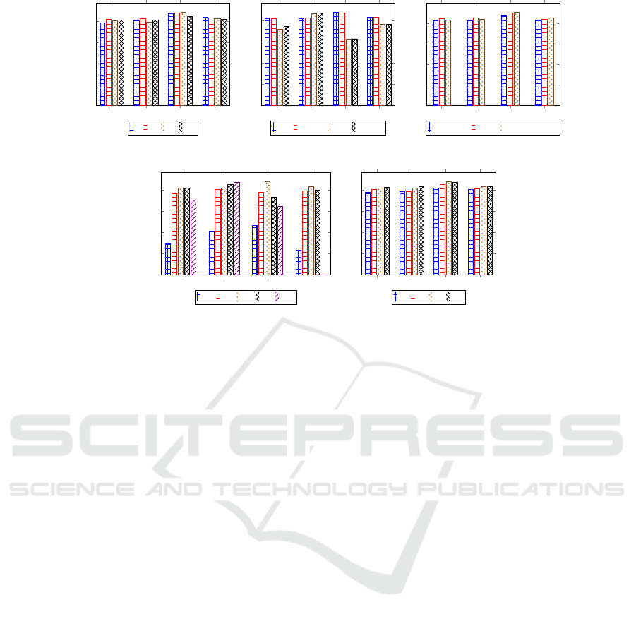
(b) Optimizer. In Figure 1, both the SGD and Nes-
terov (Sutskever et al., 2013) optimizers show a supe-
rior performance than Adam (Kingma and Ba, 2015)
or AdamW (Loshchilov and Hutter, 2019) except for
one case. The ODIN detector shows a better perfor-
mance when the optimizer is either Adam or AdamW
than when the optimizer is either SGD or Nesterov.
Specifically, it works well when CIFAR-100 is ID and
the OODs are semantically preserved datasets such as
LSUN FIX and TinyImagenet FIX.
(c) Learning Rate Scheduler. In Figure 1, cosine an-
nealing (Loshchilov and Hutter, 2017) shows a bet-
ter performance than the other two schedulers for
Baseline and ODIN. For Mahalanobis and Gram, co-
sine annealing with warm up (Loshchilov and Hut-
ter, 2017) seems to be a better choice. In case of
the CIFAR-100 ID, the optimal choice for Baseline
and ODIN is not cosine annealing but MultistepLR.
In detail, the best learning rate scheduler for each de-
tector improves the AUROC performance for every
benchmark. In particular, the best scheduler for Ma-
halanobis or Gram tends to significantly improve the
detection performance on the semantically preserved
dataset.
(d) Weight Decay. When CIFAR-10 is ID, the OOD
detection performance of the detectors varies signifi-
cantly depending on the weight decay. While the op-
timal weight decay for Mahalanobis and Gram is 5e-
4, that for Baseline is 1e-4. Surprisingly, ODIN im-
proves its OOD detection performance as the weight
decay value gets smaller. The best weight decay for
the CIFAR-100 ID is also 5e-4.
(e) Epoch. Though the OOD detection performance
gets better until epoch 300, performance drops are ob-
served in several cases as epoch reaches 400. For ex-
ample, when CIFAR-10 is ID, ODIN’s AUROC drops
on LSUN FIX when epoch changes from 300 to 400.
AUROC of the Mahalanobis and Gram detectors falls
when epoch changes from 300 to 400 to detect the
CIFAR-100 OOD. Similar tendencies are observed
when CIFAR-100 is ID.
Suggestion. One of the key observations is that
the optimal configuration for OOD detection per-
formance and classification accuracy frequently mis-
match. The following recommendations can be made:
for detecting OOD samples, the best batch size is 128,
and for the optimizer, SGD or Nesterov over Adam or
What Matters for Out-of-Distribution Detectors using Pre-trained CNN?
267
Baseline ODIN Mahalanobis Gram
50
60
70
80
90
AUROC
64 128 256 512
(a) batch size
Baseline ODIN Mahalanobis Gram
50
60
70
80
90
AUROC
SGD
Nesterov
Adam AdamW
(b) optimizer
Baseline ODIN Mahalanobis Gram
50
60
70
80
90
AUROC
MutiStepLR Cosine Cosine+WarmUp
(c) scheduler
Baseline ODIN Mahalanobis Gram
50
60
70
80
90
AUROC
1e-2 1e-3 5e-4 1e-4 1e-6
(d) weight decay
Baseline ODIN Mahalanobis Gram
50
60
70
80
90
AUROC
100 200 300 400
(e) epoch
Figure 1: CIFAR-10 AUROC performances according to the hyperparameters.
AdamW is preferred. In case of the scheduler, Multi-
StepLR is recommended for Baseline and ODIN. On
the other hand, cosine annealing with warmup is rec-
ommended for Mahalanobis and Gram. Weight de-
cay around 5e-4 is recommended for training. How-
ever, for some detector such as ODIN, this may not
be the case. Nevertheless, in most cases, weight de-
cay around 5e-4 yields the best performance. Lastly,
epoch between 300 and 400 is recommended for
training.
3.3 Hyperparameters for Network
Architecture
Study Description. The previous section consid-
ered a set of hyperparameters for training a network.
In this section, the structural hyperparameters of a
network are taken into account. First, the depth of
a network is considered. It is commonly regarded that
as the number of layers increases, the network’s clas-
sification performance gets better. To observe the cor-
relation between the number of layers and the OOD
detection capability, ResNets (He et al., 2016) with
18, 34, 50 and 101 layers are tested. Another struc-
tural hyperparameter considered in this section is the
activation function. GeLU (Hendrycks and Gimpel,
2016) is used in some of the earlier works (Hendrycks
and Gimpel, 2017). Also, ReLU (Nair and Hinton,
2010) is one of the most widely used activation func-
tions. In addition to these two activation functions, we
conduct experiments with some of the other popular
activation functions such as leaky ReLU (Maas et al.,
2013) and SiLU (Ramachandran et al., 2018).
Discussion. From the experiments that we carried
out, the deeper network does not guarantee a better
OOD detection performance contrary to the classifi-
cation accuracy. Rather, it is notable that for Base-
line and ODIN, the network with the fewest layers
performs best. Moreover, as the depth of the model
increases, both the memory usage and the computa-
tion time increase proportionally. Gram’s excessive
memory usage also hinders completing experiments
on ResNet-50 and ResNet-101.
In case of activation functions, Baseline with
ReLU and ODIN with SiLU perform slightly better
than the others. However, there seems to be no clear
winner or loser among the activation functions. On
the other hand, Mahalanobis and Gram have some
combinations that show significantly disappointing
performance. Especially, the Gram detector with all
the activation functions except for ReLU suffers from
a 50% AUROC loss. Both Mahalanobis and Gram
with all the activation functions except for ReLU spit
out a feature that contains negative values to seem-
ingly mark the anomaly score to make it difficult to
distinguish OOD from ID.
Suggestion. Even though a deeper model is pre-
ferred for the classification tasks, a shallow model is
recommended when detecting OOD samples. Also,
a light-weight model will allow more memory to be
available for the OOD detection. In addition, from
the experimental results, we learn that using ReLU as
the activation function is the best choice.
VISAPP 2022 - 17th International Conference on Computer Vision Theory and Applications
268

3.4 Classification Refinement Tricks
Study Description. Many refinement tricks have
been proposed to improve the classification accu-
racy. Label smoothing (Szegedy et al., 2016), mixup
(Zhang et al., 2018), and knowledge distillation (Hin-
ton et al., 2015) are some of those tricks. These tricks
are known to enhance model’s generalization, calibra-
tion, and classification accuracy (M
¨
uller et al., 2019;
Zhang et al., 2021; Phuong and Lampert, 2019). In
other words, they provide clearer decision boundaries
among classes of the ID samples. As the OOD detec-
tion using pre-trained CNN is aimed at improving the
OOD detection performance while largely maintain-
ing the classification accuracy, we investigate whether
these refinement tricks should help to find a clear de-
cision boundary between the ID and OOD samples.
Discussion. Each refinement trick has pros and
cons. For example, a trained model by knowledge
distillation leads to some performance improvement
with the Mahalanobis detector. On the other hand, la-
bel smoothing reveals some weakness with Baseline
and ODIN. Especially, when LSUN FIX is used as the
OOD samples, ODIN’s AUROC drops from 90.2%
to 76.5% with the CIFAR-10 ID and from 73.36%
to 60.97% with the CIFAR-100 ID. Mixup achieves
the highest AUROC with the Gram detector, but over-
all, it is not dominantly good at the OOD detection
task. Interestingly, the mixup method is the refine-
ment trick that records the best ID classification accu-
racy.
Suggestion. From the experimental result, we sug-
gest that knowledge distillation should be employed if
you want to improve both the classification accuracy
and the OOD detection performance. The other re-
finement options have cases to show pros and cons.
3.5 Designing Auxiliary Dataset
Study Description. For ODIN and Mahalanobis,
a few OOD samples called auxiliary dataset are nec-
essary. The auxiliary dataset is used when both se-
lecting T , ε (Liang et al., 2018; Lee et al., 2018b)
and tuning logistic regressors (Lee et al., 2018b). Se-
lection and tuning are conducted in such a way that
the ID set should be best distinguished from the aux-
iliary dataset. Liang et al(Liang et al., 2018) and
Lee et al(Lee et al., 2018b) used 1,000 samples of
ID and OOD each for finding the best T , ε and the
logistic regressor. However, the auxiliary dataset
may not be available, and the tuning strategy has to
be adjusted even under such circumstance. In this
section, three different tuning strategies that can be
applied without accessing the auxiliary dataset are
discussed. Adversarial, proposed by Lee et al(Lee
et al., 2018b), regards adversarial samples gener-
ated by FGSM (Goodfellow et al., 2015) as OOD.
Meanwhile, rotation and permutation are known to be
the strongest transformation methods among various
shifting transformation methods (Tack et al., 2020;
Chen et al., 2020). Therefore, Rotation and Permuta-
tion strategies regard rotated or permutated ID dataset
as OOD. We apply these three tuning strategies to
the ODIN and Mahalanobis detectors instead of their
original tuning strategies.
Discussion. For the ODIN detector, Adversarial
works well with conventional benchmarks. Mean-
while, Rotation achieves the best AUROC perfor-
mance for semantically preserved datasets. Some-
times, Rotation works even better than the ODIN’s
original tuning strategy. Even though Adversarial
does not achieve the best performance, its perfor-
mance does not fall far behind Rotation either.
For the Mahalanobis detector, Adversarial is not
the best for some cases, but overall, it shows de-
cent performance for conventional benchmarks. For
semantically preserved datasets, Rotation shows the
best performance with CIFAR-10 as ID. With CIFAR-
100 as ID, though Permutation is the best tuning strat-
egy with the semantically preserved datasets, all three
strategies show results that are too bad to be used in
practical situations.
Suggestion. As the tuning method for ODIN and
Mahalanobis, it can be suggested that Rotation should
be used as an OOD auxiliary set.
3.6 The Size of Samples in the ID
Dataset
Study Description. In general, the OOD detec-
tion capability as well as the classification accuracy is
largely affected by three factors: the distribution dif-
ference, the size of samples per class, and the num-
ber of classes. In this section, we will figure out how
the size of the training dataset (both the number of
samples and the number of classes) affects the de-
tector’s performance. In this experiment, CIFAR-10
and CIFAR-100 are used as one is ID and the other
is OOD, and vice versa. Among three factors that
affect performance, the distribution difference is not
as significant as the other two because both datasets
are originally selected from the same dataset (80 mil-
lion tiny images (Birhane and Prabhu, 2021)). To ver-
ify the effect of the other two factors, we construct a
new dataset that is made up of a partial set of CIFAR-
10, called SUBCIFAR-10. Each class in SUBCIFAR-
10 is composed of randomly picked 500 images from
CIFAR-10. With a model trained by SUBCIFAR-10,
What Matters for Out-of-Distribution Detectors using Pre-trained CNN?
269

we analyze the effect of the number of classes and the
size of samples per class on the OOD detection per-
formance.
Discussion. From the results, it turns out that the
size of samples per class is much more important than
the number of classes for the OOD detection accu-
racy. In Table 2, the effect of the number of sam-
ples in each class can be analyzed by comparing the
result on CIFAR-10 and that on CIFAR-100. When
SUBCIFAR-10 is used as the ID dataset, there is an
AUROC performance drop by up to 20% for all de-
tectors compared to the performance when the full
CIFAR-10 is used as the ID set. Comparing the case
where CIFAR-100 is used as the ID dataset with the
case where the SUBCIFAR-10 as the ID dataset, the
performance of the case with SUBCIFAR-10 falls be-
hind almost every case. This implies that the num-
ber of classes does not influence the detection perfor-
mance as much as the size of samples does for the
OOD detection.
Suggestion. Collecting more training data is an ef-
fective way to improve the OOD detection capability
regardless of all detectors. If it is impossible, increas-
ing the size of the training set through adding classes
is a decent alternative to improve the performance.
3.7 Pre-trained by Supervised
Contrastive Learning
Study Description. Hendrycks et al(Hendrycks
et al., 2019b) claimed that self-supervised learning
could improve the OOD detection capability, and sim-
ilar approaches were proposed by Tack et al(Tack
et al., 2020) and Winkens et al(Winkens et al., 2020).
In conjunction with contrastive learning, these stud-
ies successfully enhanced the OOD detection perfor-
mance. In this section, to verify the claim, the OOD
detection performance of the model pre-trained with
contrastive learning is evaluated. For a fair compari-
son, we select supervised contrastive learning (Sup-
con) (Khosla et al., 2020), trained under supervised
environment.
Discussion. Supcon achieves an impressive per-
formance improvement in Baseline and ODIN. What
we would like to emphasize in this experiment is that
Supcon is surprisingly talented at picking out OOD
samples from LSUN FIX, TinyImageNet FIX, and
CIFAR-100 when CIFAR-10 as ID. In contrast, none
of the others is capable of doing that. Nevertheless,
with the Gram detector, Supcon does not generate an
excellent result. An experiment with CIFAR-10 as ID,
LSUN FIX as OOD, AUROC drops from 84.64% to
72.6%.
Supervised contrastive learning attempts to learn
the representation where samples of the same label
are located to be closer to each other and samples of
different labels to be farther away. Therefore, when
an OOD sample is fed to the model, its representation
should not be similar to that of any ID class. This
phenomenon makes Supcon show great results with
Baseline and ODIN. On the other hand, Mahalanobis
and Gram, which already make use of features be-
tween samples for the OOD detection, are not so ben-
efited by contrastive learning.
Suggestion. Supervised contrastive learning may
be an effective alternative with a large number of data.
However, using cross-entropy loss may be a safer
choice for Mahalanobis and Gram.
4 CONCLUSION
For practical applications, distinguishing out-of-
distribution (OOD) samples from in-distribution (ID)
samples is essential for making a neural network reli-
able. In this paper, we tackled the lack of diversity of
the previous works by carrying out an extensive set of
experiments to discover the unrevealed aspects of the
OOD detection of pre-trained CNN-based models. By
conducting the OOD detection tests over 7,000 times,
we verified some of the importance factors that were
not mentioned in the previous literature. From the
extensive experimental results, various novel sugges-
tions were made. One of the interesting observations
is that pre-trained CNN-based detectors are vulner-
able to semantics-preserved OOD samples, meaning
that they do not focus on what images really mean.
We hope this study may be a solid guide for the future
OOD detection studies.
ACKNOWLEDGMENT
This work was supported by Institute of Infor-
mation & communications Technology Planning
& Evaluation (IITP) grant funded by the Korea
government(MSIT) (No.2021-0-00131, Development
of Intelligent Edge Computing Semiconductor For
Lightweight Manufacturing Inspection Equipment)
REFERENCES
Birhane, A. and Prabhu, V. U. (2021). Large image datasets:
A pyrrhic win for computer vision? In Proceedings of
the IEEE/CVF Winter Conference on Applications of
Computer Vision (WACV), pages 1537–1547.
VISAPP 2022 - 17th International Conference on Computer Vision Theory and Applications
270

Chen, T., Kornblith, S., Swersky, K., Norouzi, M., and Hin-
ton, G. E. (2020). Big self-supervised models are
strong semi-supervised learners. In Larochelle, H.,
Ranzato, M., Hadsell, R., Balcan, M. F., and Lin, H.,
editors, Advances in Neural Information Processing
Systems, volume 33, pages 22243–22255. Curran As-
sociates, Inc.
Deng, J., Dong, W., Socher, R., Li, L.-J., Li, K., and Fei-
Fei, L. (2009). Imagenet: A large-scale hierarchical
image database. In 2009 IEEE conference on com-
puter vision and pattern recognition, pages 248–255.
Ieee.
Goodfellow, I. J., Shlens, J., and Szegedy, C. (2015). Ex-
plaining and harnessing adversarial examples. In Ben-
gio, Y. and LeCun, Y., editors, 3rd International Con-
ference on Learning Representations, ICLR 2015, San
Diego, CA, USA, May 7-9, 2015, Conference Track
Proceedings.
He, K., Zhang, X., Ren, S., and Sun, J. (2016). Deep resid-
ual learning for image recognition. In Proceedings of
the IEEE conference on computer vision and pattern
recognition, pages 770–778.
Hendrycks, D. and Gimpel, K. (2016). Gaussian error linear
units (gelus). arXiv preprint arXiv:1606.08415.
Hendrycks, D. and Gimpel, K. (2017). A baseline for de-
tecting misclassified and out-of-distribution examples
in neural networks. Proceedings of International Con-
ference on Learning Representations.
Hendrycks, D., Mazeika, M., and Dietterich, T. (2019a).
Deep anomaly detection with outlier exposure. In In-
ternational Conference on Learning Representations.
Hendrycks, D., Mazeika, M., Kadavath, S., and Song,
D. (2019b). Using self-supervised learning can im-
prove model robustness and uncertainty. In Wallach,
H., Larochelle, H., Beygelzimer, A., d'Alch
´
e-Buc, F.,
Fox, E., and Garnett, R., editors, Advances in Neural
Information Processing Systems, volume 32. Curran
Associates, Inc.
Hinton, G., Vinyals, O., and Dean, J. (2015). Distilling
the knowledge in a neural network. In NIPS Deep
Learning and Representation Learning Workshop.
Hsu, Y.-C., Shen, Y., Jin, H., and Kira, Z. (2020). Gener-
alized odin: Detecting out-of-distribution image with-
out learning from out-of-distribution data. In Proceed-
ings of the IEEE/CVF Conference on Computer Vision
and Pattern Recognition, pages 10951–10960.
Khosla, P., Teterwak, P., Wang, C., Sarna, A., Tian,
Y., Isola, P., Maschinot, A., Liu, C., and Krish-
nan, D. (2020). Supervised contrastive learning. In
Larochelle, H., Ranzato, M., Hadsell, R., Balcan,
M. F., and Lin, H., editors, Advances in Neural Infor-
mation Processing Systems, volume 33, pages 18661–
18673. Curran Associates, Inc.
Kingma, D. P. and Ba, J. (2015). Adam: A method for
stochastic optimization. In Bengio, Y. and LeCun,
Y., editors, 3rd International Conference on Learn-
ing Representations, ICLR 2015, San Diego, CA, USA,
May 7-9, 2015, Conference Track Proceedings.
Krizhevsky, A. et al. (2009). Learning multiple layers of
features from tiny images.
Lee, K., Lee, H., Lee, K., and Shin, J. (2018a). Training
confidence-calibrated classifiers for detecting out-of-
distribution samples. In International Conference on
Learning Representations.
Lee, K., Lee, K., Lee, H., and Shin, J. (2018b). A simple
unified framework for detecting out-of-distribution
samples and adversarial attacks. In Proceedings of the
32nd International Conference on Neural Information
Processing Systems, pages 7167–7177.
Liang, S., Li, Y., and Srikant, R. (2018). Enhancing the reli-
ability of out-of-distribution image detection in neural
networks. In International Conference on Learning
Representations.
Loshchilov, I. and Hutter, F. (2017). SGDR: stochastic gra-
dient descent with warm restarts. In 5th International
Conference on Learning Representations, ICLR 2017,
Toulon, France, April 24-26, 2017, Conference Track
Proceedings. OpenReview.net.
Loshchilov, I. and Hutter, F. (2019). Decoupled weight
decay regularization. In International Conference on
Learning Representations.
Maas, A. L., Hannun, A. Y., and Ng, A. Y. (2013). Rec-
tifier nonlinearities improve neural network acoustic
models. In Proc. icml, volume 30, page 3. Citeseer.
M
¨
uller, R., Kornblith, S., and Hinton, G. E. (2019).
When does label smoothing help? In Wallach, H.,
Larochelle, H., Beygelzimer, A., d'Alch
´
e-Buc, F.,
Fox, E., and Garnett, R., editors, Advances in Neural
Information Processing Systems, volume 32. Curran
Associates, Inc.
Nair, V. and Hinton, G. E. (2010). Rectified linear units
improve restricted boltzmann machines. In Icml.
Netzer, Y., Wang, T., Coates, A., Bissacco, A., Wu, B., and
Ng, A. Y. (2011). Reading digits in natural images
with unsupervised feature learning. In NIPS Workshop
on Deep Learning and Unsupervised Feature Learn-
ing 2011.
Oberdiek, P., Rottmann, M., and Fink, G. A. (2020).
Detection and retrieval of out-of-distribution objects
in semantic segmentation. In Proceedings of the
IEEE/CVF Conference on Computer Vision and Pat-
tern Recognition (CVPR) Workshops.
Pacheco, A. G. C., Sastry, C. S., Trappenberg, T., Oore, S.,
and Krohling, R. A. (2020). On out-of-distribution de-
tection algorithms with deep neural skin cancer clas-
sifiers. In Proceedings of the IEEE/CVF Conference
on Computer Vision and Pattern Recognition (CVPR)
Workshops.
Phuong, M. and Lampert, C. (2019). Towards under-
standing knowledge distillation. In Chaudhuri, K.
and Salakhutdinov, R., editors, Proceedings of the
36th International Conference on Machine Learning,
volume 97 of Proceedings of Machine Learning Re-
search, pages 5142–5151. PMLR.
Ramachandran, P., Zoph, B., and Le, Q. V. (2018). Search-
ing for activation functions.
Sastry, C. S. and Oore, S. (2020). Detecting out-of-
distribution examples with gram matrices. In Interna-
tional Conference on Machine Learning, pages 8491–
8501. PMLR.
What Matters for Out-of-Distribution Detectors using Pre-trained CNN?
271

Shafaei, A., Schmidt, M., and Little, J. J. (2019). A less
biased evaluation of out-of-distribution sample detec-
tors. In 30th British Machine Vision Conference 2019,
BMVC 2019, Cardiff, UK, September 9-12, 2019,
page 3. BMVA Press.
Sutskever, I., Martens, J., Dahl, G., and Hinton, G. (2013).
On the importance of initialization and momentum in
deep learning. In Dasgupta, S. and McAllester, D.,
editors, Proceedings of the 30th International Confer-
ence on Machine Learning, volume 28 of Proceedings
of Machine Learning Research, pages 1139–1147, At-
lanta, Georgia, USA. PMLR.
Szegedy, C., Vanhoucke, V., Ioffe, S., Shlens, J., and Wo-
jna, Z. (2016). Rethinking the inception architecture
for computer vision. In Proceedings of the IEEE Con-
ference on Computer Vision and Pattern Recognition
(CVPR).
Tack, J., Mo, S., Jeong, J., and Shin, J. (2020). Csi: Nov-
elty detection via contrastive learning on distribution-
ally shifted instances. In Larochelle, H., Ranzato,
M., Hadsell, R., Balcan, M. F., and Lin, H., editors,
Advances in Neural Information Processing Systems,
volume 33, pages 11839–11852. Curran Associates,
Inc.
Winkens, J., Bunel, R., Roy, A. G., Stanforth, R., Natara-
jan, V., Ledsam, J. R., MacWilliams, P., Kohli, P.,
Karthikesalingam, A., Kohl, S., et al. (2020). Con-
trastive training for improved out-of-distribution de-
tection. arXiv preprint arXiv:2007.05566.
Yu, F., Zhang, Y., Song, S., Seff, A., and Xiao, J. (2015).
Lsun: Construction of a large-scale image dataset us-
ing deep learning with humans in the loop. arXiv
preprint arXiv:1506.03365.
Yu, Q. and Aizawa, K. (2019). Unsupervised out-of-
distribution detection by maximum classifier discrep-
ancy. In Proceedings of the IEEE/CVF International
Conference on Computer Vision, pages 9518–9526.
Zhang, H., Cisse, M., Dauphin, Y. N., and Lopez-Paz, D.
(2018). mixup: Beyond empirical risk minimization.
In International Conference on Learning Representa-
tions.
Zhang, L., Deng, Z., Kawaguchi, K., Ghorbani, A., and
Zou, J. (2021). How does mixup help with robust-
ness and generalization? In International Conference
on Learning Representations.
APPENDIX
Detailed Explanation of Compared Detectors with
Pre-trained CNNs
ODIN. makes use of perturbation noise gener-
ated by the FGSM method that back-propagates the
gradients of values after softmax, S
ˆy
. However, it is
different in the sense that only its sign is used and
then −ε is multiplied. The method to make perturbed
inputs is as follows:
˜x = x − εsign(−∇
x
S
ˆy
(x;T )) (1)
After the perturbed input ˜x is passed through the net-
work, temperature scaling is applied by dividing log-
its f (x) by temperature T . Temperature scaling for
input x is as follows:
S(x; T ) =
exp( f (x)/T )
∑
C
j=1
exp( f
j
(x)/T )
, (2)
where C is the number of classes and T denotes
temperature for scaling.
In our experiments, candidates for T and ε are [1,
10, 100, 1000] and [0, 0.0005, 0.001, 0.0014, 0.002,
0.0024, 0.005, 0.01, 0.05, 0.1, 0.2], respectively.
Mahalanobis. defines the Mahalanobis scores based
on the Mahalanobis distance. To measure the Maha-
lanobis distance, empirical class mean ˆµ
c
and covari-
ance
ˆ
Σ of training samples {(x
1
,y
1
),. .., (x
N
,y
N
)} are
calculated for every layer as:
ˆµ
c
=
1
N
c
∑
f (x
i
),
ˆ
Σ =
1
N
∑
c
∑
i:y
i
=c
( f (x
i
) − ˆµ
c
)( f (x
i
) − ˆµ
c
)
T
,
(3)
where N
c
is the number of training samples with
label c.
After calculating the class mean and covariance, Ma-
halanobis defines confidence score M(x) at every
layer using the Mahalanobis distance between test
sample x and the closest class-conditional Gaussian
distribution as:
M(x) = max
c
−( f (x) − ˆµ
c
)
T
ˆ
Σ
−1
( f (x) − ˆµ
c
) (4)
To tune logistic regression parameters and ε, a few
ID and OOD samples are necessary. Here are the
candidates for ε: [0, 0.0005, 0.001, 0.0014, 0.002,
0.0024, 0.005, 0.01, 0.05, 0.1, 0.2].
Gram. calculates the p-th order Gram matrix G
p
l
with
feature map F
l
for every layer l. Then, correlations for
any image are obtained through the Gram matrix as:
G
p
l
= (F
p
l
F
p
l
T
)
1
p
(5)
With the Gram matrix, the class-specific minimum
and maximum feature correlations are stored in an ex-
ternal memory. The deviation of a test image can be
computed as:
δ(min,max,value) =
0 i f min ≤ value ≤ max
min−value
|min|
i f value < min
value−max
|max|
i f value > max
(6)
VISAPP 2022 - 17th International Conference on Computer Vision Theory and Applications
272

(a) LSUN (b) TinyImagenet
Figure 2: Semantic-damaged datasets. These datasets are generated by applying OpenCV’s image processing.
(a) LSUN FIX (b) TinyImagenet FIX
Figure 3: Semantics-preserved datasets. These datasets are generated by applying torchvision.transforms.Resize().
where value in equation 6 denotes the value appeared
in the test image’s Gram matrix.
Transformation with Semantics-preservation.
Originally, the size of the LSUN images is uniformly
256 × 256 while the images in ImageNet have various
sizes. The LSUN and TinyImagenet datasets are
resized to fit to the model’s input size as provided by
Liang et al(Liang et al., 2018). According to Tack
et al(Tack et al., 2020), conventional benchmarks
(LSUN, TinyImagenet) contain artificial noise in-
serted by the OpenCV library’s image processing. It
seems that the semantics in the LSUN and TinyIm-
agenet datasets are significantly damaged. So, it is
hard to recognize the picture correctly. To overcome
such issue, revised datasets such as LSUN FIX,
TinyImageNet FIX are generated by the PyTorch
torchvision.transforms.Resize() operations
that conduct both resizing and bilinear interpolation.
Through this, the datasets preserve image semantics
better than the original datasets while their resolution
remains the same. This is what we call semantics-
preserved transformation.(See Figure 2 and 3).
Baseline Settings. For fair comparisons, we have se-
lected the most commonly used options for the OOD
detection task. The ResNet with 18 layers with the
ReLU activation function is adopted as the model ar-
chitecture. The network is trained with a batch nor-
malization with no dropout. The model is trained for
300 epochs with a batch size of 128, the SGD op-
timizer with 0.9 momentum, 5e-4 weight decay and
0.1 learning rate which decays by a factor of 10 at
{0.5×epoch, 0.75×epoch}. Each input is flipped ran-
domly with a probability of 0.5, padded with edge
pixels by one eighth of the size of the input, then
clipped at random locations. Losses are calculated
by the cross-entropy loss. Models with the best val-
idation set accuracy were stored during the training
process.
What Matters for Out-of-Distribution Detectors using Pre-trained CNN?
273
