
Unidentified Floating Object Detection in Maritime Environment
Darshan Venkatrayappa
1
, Agn
`
es Desolneux
1
, Jean-Michel Hubert
2
and Josselin Manceau
2
1
Centre Borelli, ENS Paris-Saclay, Gif-sur-Yvette, France
2
iXblue, Saint-Germain-en-Laye, France
Keywords:
Floating Object Detection, Unsupervised Learning, Self-similarity.
Abstract:
In this article, we present a new unsupervised approach to detect unidentified floating objects in the mar-
itime environment. The proposed approach is capable of detecting floating objects online without any prior
knowledge of their visual appearance, shape or location. Given an image from a video stream, we extract the
self-similar and dissimilar components of the image using a visual dictionary. The dissimilar component con-
sists of noise and structures (objects). The structures (objects) are then extracted using an a contrario model.
We demonstrate the capabilities of our algorithm by testing it on videos exhibiting varying maritime scenarios.
1 INTRODUCTION
In the maritime environment, one can encounter two
categories of floating objects. The first category in-
volves military and commercial ships, boats, trolleys,
small buoys etc. The second category called Uniden-
tified Floating Objects (UFOs) include objects like
drifting containers, drifting iceberg, drifting cargo
boxes, driftwood, debris etc. These UFOs are ran-
dom, diverse, rare and are a threat to maritime trans-
portation. To limit the risk in the maritime domain,
there is a need to detect and track the floating ob-
jects and particularly the UFOs. From a century ago
until recently, ranging devices such as Lidar, radar
(Onunka and Bright, 2010) and sonar (Heidarsson
and Sukhatme, 2011) have been used to counter the
above-mentioned risky scenarios. But, Lidar is ex-
pensive and radar data is sensitive to the variation in
the climate, the shape, size, and material of the tar-
gets. As a result, the ranging devices have to be sup-
plemented by other sensors such as cameras for de-
tecting UFOs.
To tackle the limitations of ranging devices, the
computer vision community has resorted to camera-
based object detection and tracking. Several re-
searchers (Bloisi et al., 2014), (Heidarsson and
Sukhatme, 2011), (Prasad et al., 2017) have used
camera or a combination of camera and ranging de-
vice for floating object detection. We can find a
detailed description about the challenges and differ-
ent sensors used in the maritime scenario in (Prasad
et al., 2017). Most of the state-of-the-art Back-
ground Subtraction (BS) algorithms (St-Charles and
Bilodeau, 2014), (St-Charles et al., 2014), (Oliver
et al., 2000),(Elgammal et al., 2000), (Sobral and Va-
cavant, 2014) etc. that address dynamic backgrounds
have been used in the maritime domain. A review
of different background subtraction algorithms used
in maritime object detection can be found in (Prasad
et al., 2019).
The authors of (Socek et al., 2005) propose
a Bayesian decision framework based hybrid fore-
ground object detection algorithm in the maritime do-
main. Kristan et al. (Kristan et al., 2015) use Gaus-
sian Mixture Model (GMM) to segment water, land
and sky regions. The GMM relies on the availabil-
ity of the precomputed priors using training data. The
major drawback of this method is the expensive pre-
training step. The Authors of (Bloisi and Iocchi,
2012) propose a non-parametric Background Subtrac-
tion method for the maritime scenario using a 3 step
approach consisting of online clustering, background
update and noise removal. The problem with these
methods is that most of them fail with varying back-
ground or lighting conditions and the ones that suc-
ceed are computationally very expensive. The au-
thors of (Sobral et al., ) and (Karnowski et al., 2015)
use Robust Principal Components Analysis (RPCA)
to detect and track sailboats and dolphins respectively.
Most of the methods based on low rank and sparse
representation are not suitable for real-time applica-
tions as they are highly complex and require a col-
lection of frames to detect the object. With the ad-
vent of deep learning, many new supervised mod-
els (Moosbauer et al., 2019), (Bovcon and Kristan,
2020), (Yang et al., 2019), (Lee et al., 2018) have been
proposed for floating object detection in general and
ship detection in particular. An evaluation of different
Venkatrayappa, D., Desolneux, A., Hubert, J. and Manceau, J.
Unidentified Floating Object Detection in Maritime Environment.
DOI: 10.5220/0010771800003124
In Proceedings of the 17th International Joint Conference on Computer Vision, Imaging and Computer Graphics Theory and Applications (VISIGRAPP 2022) - Volume 5: VISAPP, pages
65-74
ISBN: 978-989-758-555-5; ISSN: 2184-4321
Copyright
c
2022 by SCITEPRESS – Science and Technology Publications, Lda. All rights reserved
65

Figure 1: Workflow.
deep semantic segmentation networks for object de-
tection in maritime surveillance can be found in (Cane
and Ferryman, 2018). Most of the supervised and un-
supervised deep learning methods for object detection
require a large amount of training data and in our case
data is sparse as we have no prior knowledge about the
UFO encountered in the ocean. One of the advantage
of our method is it considers the current frame as the
training data.
In the far sea scenario, the background (sea and
sky) have their respective color and texture. Float-
ing objects can be detected by separating the back-
ground from the object. Our approach can be con-
sidered as zero-shot internal learning (Shocher et al.,
2018) without a neural network. We detect the mar-
itime objects by removing the self-similar component
from the image. The self-similar component(self-
similar image) is obtained using a visual dictionary.
The dissimilar component(dissimilar image) is then
the difference between the original image and the self-
similar component. Thus, the self-similar component
of the image is removed and the dissimilar image is
left with the noise and structures (objects). The noise
and the structures can be separated by statistical tests
based on an a contrario approach (Desolneux et al.,
2008). Our algorithm works on the dissimilar com-
ponent at different scales. This work mainly concen-
trates on detecting floating objects in the far sea using
a camera mounted on a ship. That being said, our al-
gorithm performs well near the shore with a camera
onshore and is able to detect big, small, far and near
objects in the sea at different climatic conditions. Our
method can also be used to detect trash floating on
rivers and canals. It is to be noted that here, we are
not concerned with labeling or classifying the object
as boat, ship, cargo container, etc. instead, we assume
that any floating object and in particular the UFOs are
obstacles and needs to be detected. Our work is more
of an early warning system.
2 WORKFLOW
The workflow of the proposed algorithm is shown in
Fig. 1. Let y be an original image obtained during the
image acquisition process (Fig. 2a). We are interested
in a self-similar image ˆx (Fig. 2b), where each of its
patches admits a sparse representation in terms of a
learned dictionary (Elad and Aharon, 2007). For each
pixel position (i, j) of the image y, we denote by R
i j
y
the size n column vector formed by the gray-scale lev-
els of the squared
√
n ×
√
n patch of the image y and
the top-left corner of the patch is represented by the
coordinates (i, j). The goal is to learn a dictionary
ˆ
D
(Fig. 2e) of size n ×k, with k ≥ n and whose columns
are normalized. Here, an initialization of the dictio-
nary denoted by D
init
(Fig. 2d) is required which is
done using random patches from the original image
y. We learn
ˆ
D using the K-SVD algorithm (Lebrun
and Leclaire, 2012) and use the learnt
ˆ
D to obtain the
self-similar image.
In the first step, we use the fixed dictionary
ˆ
D to
compute the sparse approximation
ˆ
α of all the patches
R
i j
y of the image in
ˆ
D. i.e. for each patch R
i j
y a col-
umn vector
ˆ
α
i j
of size k is built such that it has only a
few non-zero coefficients and such that the distance
between R
i j
y and its sparse approximation
ˆ
D
ˆ
α
i, j
is
very small.
Argmin
ˆ
α
i j
k
ˆ
α
i j
k
0
such that kR
i j
y −
ˆ
D
ˆ
α
i j
k
2
2
≤ ε
2
(1)
Where k
ˆ
α
i j
k
0
refers to the number of non-zero co-
efficients of
ˆ
α
i j
also known as l
0
norm of
ˆ
α
i j
. This
is a NP hard problem, and we make use of Orthog-
onal Recursive Matching Pursuit (ORMP) to get an
approximate solution. In Eq. (1), ε is used during the
break condition of the ORMP,
ˆ
D is of size n ×k,
ˆ
α
i j
is a column vector of size k ×1 and R
i j
y is a column
vector of size n ×1. In the second step, we update
the columns of the dictionary
ˆ
D one by one, to reduce
the quantity in Eq. (2) without increasing the spar-
sity penalty
ˆ
α
i j
such that all the patches in the image
y are efficient. This is achieved using the K-SVD al-
gorithm. More details about K-SVD can be found in
(Lebrun and Leclaire, 2012).
∑
i, j
k
ˆ
D
ˆ
α
i j
−R
i j
yk
2
2
(2)
We repeat the above two steps for some iterations
say K iter. Once these K iter iterations are done,
each patch R
i j
y of the image y corresponds to the self-
similar version
ˆ
D
ˆ
α
i j
. In the third and final step, we
reconstruct the complete self-similar image from all
the self-similar patches by solving the minimization
VISAPP 2022 - 17th International Conference on Computer Vision Theory and Applications
66

(a) (b) (c) (d) (e)
Figure 2: (a). Original image y, (b). self-similar component ˆx, (c). dissimilar component r (contrast and brightness adjusted),
(d). Random patches from y used to learn the dictionary, (e). Final learnt dictionary
ˆ
D. These image are obtained by using
the dictionary of size 512 and patch size 64 (8x8).
problem in Eq. (3). First term in Eq. (3) represents a
fidelity term which controls the global proximity to
our reconstruction ˆx with the input image y . The
second term controls the proximity of the patch R
i j
ˆx
of our reconstruction to Dα
i j
(Lebrun and Leclaire,
2012).
ˆx = Argmin
x∈IR
N
λkx −yk
2
2
+
∑
i, j
k
ˆ
D
ˆ
α
i j
−R
i j
yk
2
2
(3)
We extend the above algorithm to colour images by
concatenating the R,G,B values of the patch to a sin-
gle column. Thus the algorithm learns the correlation
between the color channels resulting in a better update
of the dictionary. The dissimilar component r (Fig.
2c) is extracted by taking the pixel-wise difference be-
tween y and ˆx as in r(i, j,ch) = y(i, j,ch)− ˆx(i, j, ch).
Where, i, j and ch represents the pixel coordinates and
the channel number respectively. Thus obtained dis-
similar image contains only noise and structures (ob-
jects) as it is free from self-similar component. The
intuition is that it is straightforward to detect salient
regions/objects in the dissimilar image compared to
detection in the original image y. We use a multi-scale
approach to detect the structures of different sizes.
We follow (Lowe, 2004) to obtain images at differ-
ent scales and learn individual dictionary for each of
the scaled version of the original image. Finally, we
construct the dissimilar image at different scales, as
previously explained.
2.1 Object Detection and Localization
The a contrario detection theory was primarily pro-
posed by (Desolneux et al., 2008) and has been suc-
cessfully employed in many computer vision applica-
tions such as shape matching (Mus
´
e et al., 2003), van-
ishing point detection (Lezama et al., 2017), anomaly
detection (Davy et al., 2018), spot detection (Gros-
jean and Moisan, 2009) etc. The a contrario frame-
work is based on the probabilistic formalization of
the Helmholtz perceptual grouping principle. Ac-
cording to this principle, perceptually meaningful
structures represent large deviations from random-
ness/naive model. Here, the structures to be detected
are the co-occurrence of several local observations
(Desolneux et al., 2008).
We define a naive model by assuming that all lo-
cal observations are independent. By using this a
contrario assumption, we can compute the probability
that a given structure occurs. More precisely, we call
the number of false alarms (NFA) of a structure con-
figuration, its expected number of occurrences in the
naive model. We say that a structure is ε-meaningful
if its NFA is smaller than ε. The smaller the ε, the
more meaningful the event. Given a set of random
variables (U
i
)
i∈[|1,N|]
with observed values (u
i
)
i
, we
define the NFA of each observation as NFA(u,i) :=
NP(U
i
≥u
i
),(Eq.(4)) where P is the a contrario prob-
ability distribution (white noise in general). Here N is
the total number of tests, which is nothing but the total
number of pixels in all the images at different chan-
nels and scales. We will apply this NFA to u being
the dissimilar component, and the naive model is con-
structed in such a way that each pixel of the dissimilar
image follows a standard normal distribution.
We aim to detect structures in the dissimilar image
r. The dissimilar image r is unstructured, similar to a
coloured noise and not necessarily Gaussian. A care-
ful study of the distribution of the dissimilar image
shows that it follows a generalized Gaussian distribu-
tion (Davy et al., 2018). A non-linear transform is
used to re-scale the dissimilar image to fit a centred
Gaussian distribution with unit variance. This cen-
tered Gaussian distribution with unit variance is con-
sidered as the naive model. The naive model doesn’t
require the noise to be uncorrelated. Since structures
are expected to deviate from this naive model, this
amounts to checking the tails of the Gaussian and to
retain high values as significant if their tail has a very
small area. Similar to (Grosjean and Moisan, 2009),
we convolve the dissimilar image with a kernel K
c
of
given radius, which results in a new image r = r ∗K
c
.
Thus obtained r is normalized to have a unit vari-
ance. As we have assumed the dissimilar component
Unidentified Floating Object Detection in Maritime Environment
67

Table 1: Dataset and its properties.
Seq Name Number of frames Resolution Time taken(sec) Details Camera
S.1 Ship-wreckage 257 1276 x 546 10 Wreckage from a broken ship On-board, camera motion
S.2 Floating-Container 300 640 x 352 3 Containers floating in sea On-board, camera motion
S.3 Sinking-Trolley 381 1920 x 1080 28 Debris of varying size On-board, camera motion
S.4 Space-capsule 257 1276 x 438 9 Space capsule being retrieved back On-board, no camera motion
S.5 MVI 1644 VIS 252 1920 x 1080 28 From SMD (Prasad et al., 2017), contains big ships On-shore, no motion
S.6 Rainy 250 1920 x 1080 28 Rainy and windy condition camera motion
S.7 MVI 0788 VIS 299 1920 x 1080 28 From SMD (Prasad et al., 2017), Far and small objects Sever camera motion
to be a stationary Gaussian field, the result after fil-
tering is also Gaussian. We use N
k
= 3 number of
disks with radius 1,2 and 3 at each scale to detect the
salient structures in the dissimilar image. We detect
the structures on both the tail of the distribution using
the NFA given in Eq.(4). The number of tests in our
case is given by N = N
k
×N
ch
×
∑
N
scale
−1
0
|Ω
s
|. Here,
N
k
refers to the number of disk kernels, N
ch
refers to
the number of channels, N
scale
is the number of scales
used and Ω is the set of pixels in the dissimilar image
at a given scale.
By using the above approach, structures are de-
tected at a certain radius of the kernel. Using the
center and the radius of detection, we construct a
square bounding box. Many of these bounding boxes
overlap. We use the opencv function such as ”find-
Contours” and ”approxPolyDP” to fuse the overlap-
ping bounding boxes and get a single big rectangular
bounding box. Thus obtained bounding boxes have
many false detection due to spurious dynamics of wa-
ter. One of the easiest ways to refine false detection is
to ignore the bounding box which has no key-points
present in it. A combination of key-points from SIFT
(Lowe, 2004) and SURF (Bay et al., 2008) detectors
are used as they provide a good coverage of the im-
age space, including corners, edges and textured ar-
eas. In our case, we make use of 200 most dominant
key-points from each of the detectors to refine false
detection. Another approach to refine false detection
is to track all the detected pixels for a few frames. De-
tections on the water(false detections) loose the track
where as majority of the detections on the object are
tracked correctly. The tracks fail in case of camera
motion or motion of the boat as in video sequence 7.
3 EXPERIMENTS AND RESULTS
In the dictionary learning part, we set the patch size n
to 16 and the size of the dictionary k is fixed to 128.
The break condition for ORMP ε is set to 10
−6
. The
number of iterations in the K-SVD process K iter is
fixed to 7. λ in Eq(3) is set to 0.15. These parameters
are choosen emperically as they give a good trade-off
between the size of the detected object and the speed
of the algorithm. More details about these parameters
can be found in (Lebrun and Leclaire, 2012). In the
a contrario detection part, we have experimented with
both ε=10
2
(or logε = 2) and ε = 10
−2
(or logε= −2)
where logε is the logarithm of ε. N
scales
represents the
number of scales used in the multi-scale approach and
set to 4. The Radius of the circular kernel K
c
= 1,2,3.
All the parameters are empirically chosen. In the mar-
itime object detection scenario, only a few data-sets
have been proposed and most of these data-sets are
intended for ship detection. As the UFOs are random
and sporadic, it is very difficult to come up with a
database/data-set and there is hardly any dataset avail-
able. Here, we introduce a small data-set by extract-
ing portion of videos from YouTube. We manually
annotate the dataset by drawing ground truth bound-
ing boxes around the object. To demonstrate the ca
pabilities of our algorithm to detect ships/boats in the
sea, we make use of the Singapore maritime dataset
(Prasad et al., 2017). The features of our data-set are
tabulated in Table 1.
The algorithm was coded in C++ using OpenCV
library and tested on a laptop with 8 cores. The av-
erage time taken (in seconds) for each frame of the
sequence is given in the 5th column of Table 1. In our
experiments, the dictionary is learnt for every frame.
Real time performance can be achieved by initially
using a pre-learnt dictionary and then learning the dic-
tionary (online and in parallel) for every M duration
of time. Most of the modern CNN based object de-
tection methods outperform our method as they are
completely supervised in nature. Our approach is un-
supervised. So, we compare our method with unsu-
pervised traditional methods. As our method sepa-
rates the self-similar and the dissimilar content to de-
tect the object it can be considered as a background
subtraction method.
In the maritime object detection literature some
authors have used saliency methods for comparison.
So, The results of our algorithm are compared with
i) Two Background Subtraction (BS) methods: SuB-
SENSE and LOBSTER. ii) Two saliency detection
methods: spectral Residual Approach (SRA) (Hou
and Zhang, 2007) and ITTI (Itti et al., 1998). The
code for SRA and ITTI can be found in (Hou and
Zhang, 2007) and (Walther and Koch, 2006). The
code for SuBSENSE (St-Charles et al., 2014) and
LOBSTER (St-Charles and Bilodeau, 2014) can be
VISAPP 2022 - 17th International Conference on Computer Vision Theory and Applications
68

Table 2: Quantitative Evaluation : DR: Detection Rate, FAR: False Alarm Rate.
logε=-2 logε=2 IITI SRA LOBSTER SuBSENSE
Seq DR FAR DR FAR DR FAR DR FAR DR FAR DR FAR
1 0.701 0.080 0.853 0.124 0.434 0.493 0.707 0.383 0.53 0.467 0.494 0.754
2 0.813 0.026 0.934 0.010 0.683 0.023 0.682 0.201 0.8353 0.067 0.743 0.092
3 0.552 0,142 0.688 0,371 0.118 0.274 0.501 0.487 0.446 0.875 0.622 0.792
4 0.891 0.167 0.921 0.199 0.379 0.601 0.876 0.402 0.863 0.523 0.190 0.080
5 0.531 0.074 0.512 0.193 0.621 0.234 0.689 0.523 0.23 0.79 < 0.0001 0.998
6 0.793 0.312 0.988 0.507 0.972 0.401 0.754 .748 0.17 0.977 0.536 0.949
7 0,653 0,464 0,874 0,542 0,514 0,724 0,538 0,741 0,584 0,928 0,354 0,836
found in (Sobral, 2013). For all the four methods, we
have used the default parameters provided by the au-
thors. Fig. 3, Fig. 4 and Fig. 5 presents the qualitative
comparison of the methods for some of the videos.
The red and green bounding boxes present in the 2nd
row of each layer in Fig. 3 represent the detections ob-
tained by our algorithm with logε = 2 and logε = −2
respectively. The bounding boxes in orange and pink
in the 3rd row of each layer in Fig. 3 belong to ITTI
and SRA, respectively. LOBSTER and SuBSENSE
methods are shown in 4th and 5th rows respectively.
False detections from our approach are shown in Fig.
6. The detections with logε = 2 takes into account
many weak detections, meaning it detects many pix-
els as part of the object and this results in a red bound-
ing box which is sometimes much bigger than the ob-
ject itself. The detection with logε = −2 takes into
account only the robust detections, meaning a small
number of pixels are detected as part of an object and
this results in a green bounding box which is usually
smaller than the object. An object can contain many
of these small green bounding boxes. Thus by varying
the logε, we can control the number of false alarms.
Lower the logε, the stronger and accurate the detec-
tions are. Both SRA and ITTI result in many false
detections. In our experiments, varying the patch size
and dictionary size increases the algorithm run-time
with minor improvements in the detection results.
Quantitative evaluation is performed by calculat-
ing the True Positive TP (If a bounding box is present
on the Ground truth object), False Positive FP (If we
detect an object when there is none) and False Neg-
ative FN (If we fail to detect the Ground truth ob-
ject). Using these three measures, we further calcu-
late the Detection Rate (DR = TP/(TP + FN)) and
False Alarm Rate (FAR = FP/(TP + FP)). Ideally,
DR should be high, whereas the FAR should be as
low as possible.
Most of the supervised object detection ap-
proaches use Intersection over Union (IOU) as a met-
ric to evaluate performance. As our approach is un-
supervised, we don’t get a complete detection of the
object. Some objects are completely detected and oth-
ers may have multiple BB’s detecting different parts
of the same object. Additionally, our approach us-
ing logNFA = −2 prioritises the most salient parts
of the object. So, the IOU metric is not suitable for
our application. Similar to (Shin et al., 2015), for ev-
ery frame in a sequence, we check for the presence
of detected Bounding Box(BB) on the ground truth
(GT) object. If the detected BB has more than 30%
overlap with the ground truth we consider it as a True
Positive(TP). In some cases multiple BB’s may be de-
tected on a single GT object. In such a scenario, we
fuse the areas of the BB’s and if the fused area is more
than 30% of the ground truth BB then we consider it
as TP. A FP is detected if a BB is present in the back-
ground (sea, sky or land) and a FN is detected if the
Ground truth object doesn’t contain any detected BB.
Thus, for a given video sequence the final value of FP,
FN and TP is obtained by accumulating scores across
all the frames of the sequence.
The quantitative results of our experiments are
tabulated in Table 2. From this table, it is evident that
our algorithm with logε = −2 gives minimum FAR
for 5 of the video sequences. As logε = −2 takes
into account only the robust detections, we can ex-
pect the FAR to be minimum, thus reducing the false
alarms. This is also a reason for our algorithm with
logε = −2 to have more FN compared to logε = 2. For
most of the video sequence, maximum DR is achieved
by our algorithm with logε = 2, as it takes into ac-
count both strong and weak detections. Thus, our al-
gorithms outperforms the other algorithm for most of
the video sequence. We have compared our algorithm
with many other BS methods provided by (Sobral,
2013). But, here in this paper we show the results
for 2 prominent BS methods. Most of the BS meth-
ods fail due to camera motion, which is often the case
in onboard maritime scenario. LOBSTER method ex-
hibits lower FAR compared to SuBSENSE. The two
saliency methods perform weakly in detecting small
objects but perform better than the two BS methods.
Unidentified Floating Object Detection in Maritime Environment
69
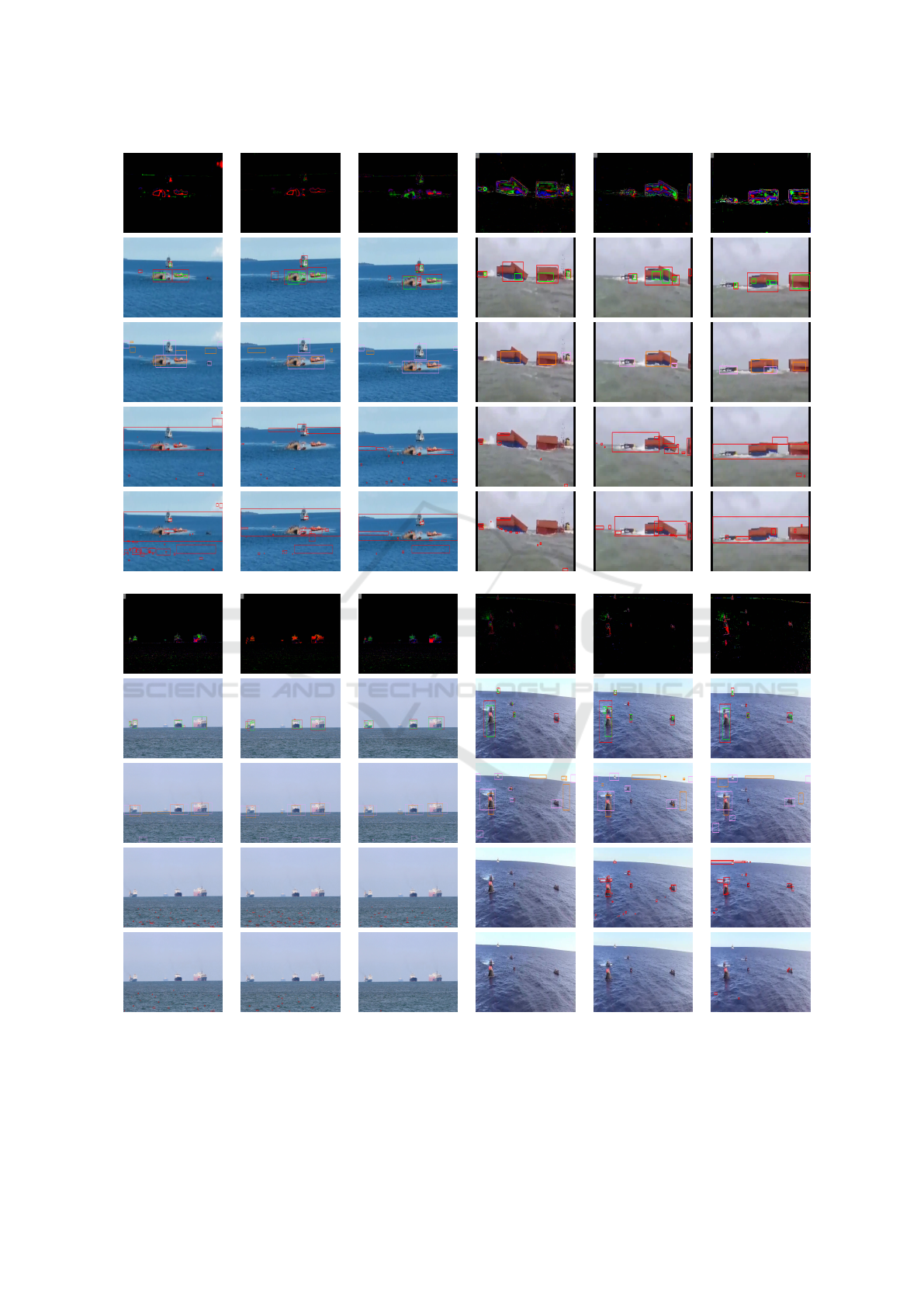
S.1(39) S.1(97) S.1(149) S.2(6) S.2(50) S.2(105)
S.5(8) S.5(19) S.5(38) S.4(3) S.4(67) S.4(158)
Figure 3: Qualitative results : The sequence number and frame numbers are indicated below each of the image. Top row of
each layer represents the dissimilar image (contrast and brightness adjusted). 2nd row of each layer indicates the detection
made by our algorithm with logε=2 (Red bounding boxes) and logε=−2 (Green bounding boxes). Detections in the 3rd row
of each layer belongs to ITTI (Orange bounding boxes) and SRA (Pink bounding boxes). 4th and 5th row shows the results
from LOBSTER and SuBSENSE respectively.
VISAPP 2022 - 17th International Conference on Computer Vision Theory and Applications
70
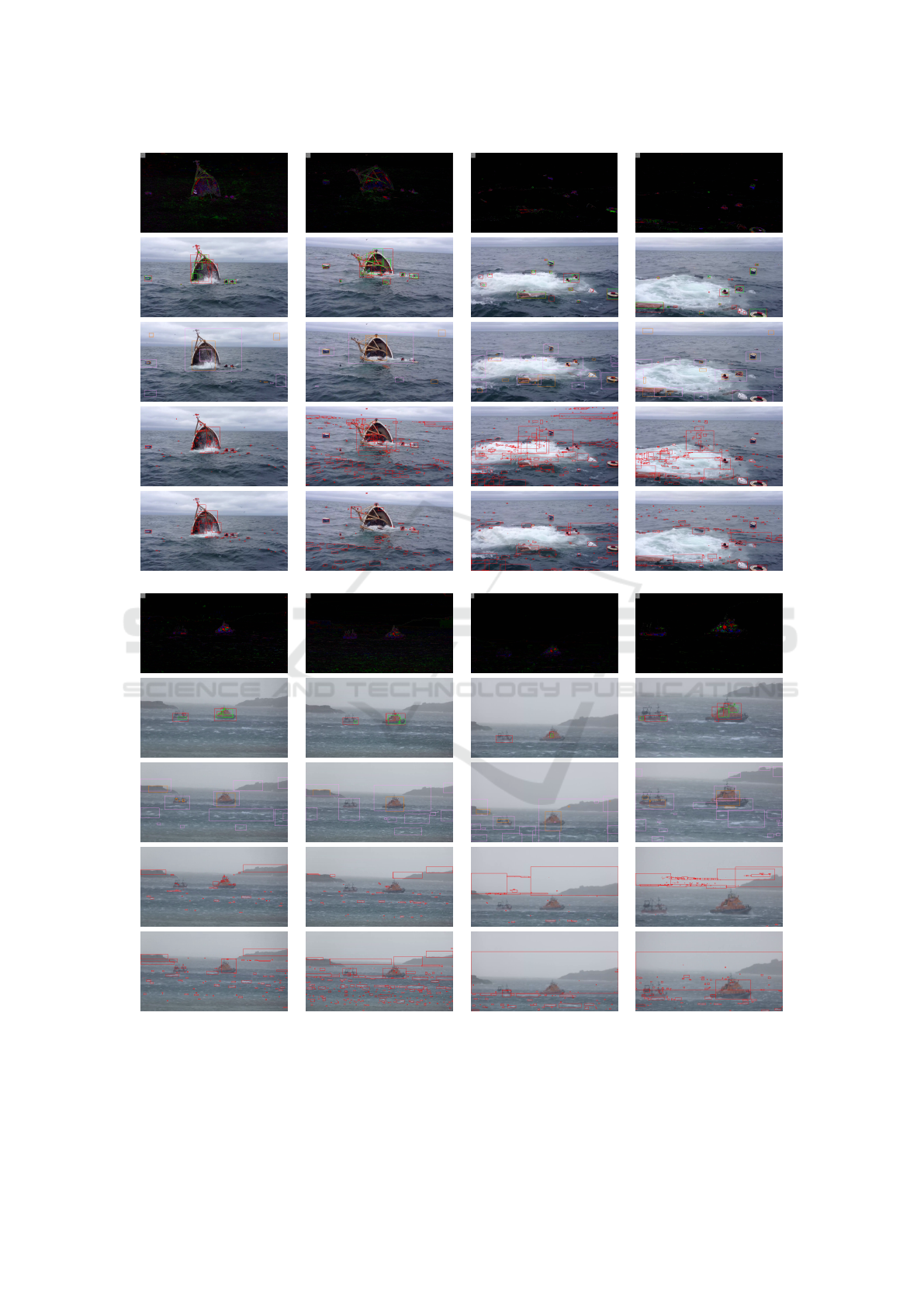
S.3(1) S.3(88) S.3(273) S.3(358)
S.6(41) S.6(104) S.6(195) S.6(246)
Figure 4: Qualitative results : The sequence number and frame numbers are indicated below each of the image. Top row of
each layer represents the dissimilar image (contrast and brightness adjusted). 2nd row of each layer indicates the detection
made by our algorithm with logε=2 (Red bounding boxes) and logε=−2 (Green bounding boxes). Detections in the 3rd row
of each layer belongs to ITTI (Orange bounding boxes) and SRA (Pink bounding boxes). 4th and 5th row shows the results
from LOBSTER and SuBSENSE respectively.
Unidentified Floating Object Detection in Maritime Environment
71
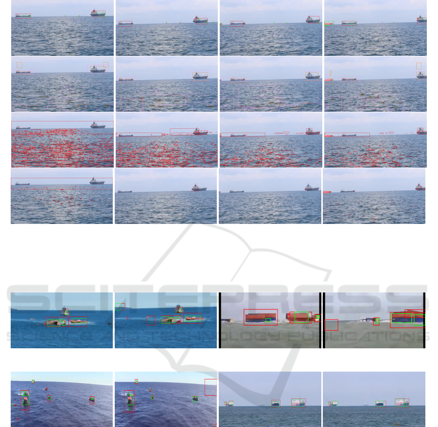
(a) S.7(47) (b) S.7(67) (c) S.7(166) (d) S.7(231)
Figure 5: Qualitative results : The sequence number and frame numbers are indicated below each of the image. First row
indicates the detection made by our algorithm with logε=2 (Red bounding boxes) and logε=−2 (Green bounding boxes).
Detections in the 2nd row of each layer belongs to ITTI (Orange bounding boxes) and SRA (Pink bounding boxes). 3rd and
4th row shows the results from LOBSTER and SuBSENSE respectively.
(a) S.1(52) (b) S.1(110) (c) S.2(132) (d) S.2(270)
(e) S.4(64) (f) S.4(129) (g) S.5(127) (h) S.5(157)
Figure 6: Qualitative results: False detections resulting from our approach. Sequence number and frame number are below
each image.
4 CONCLUSION AND FUTURE
WORK
We have proposed an unsupervised floating object de-
tection algorithm specific to the maritime environ-
ment. The effectiveness of our approach was demon-
strated on challenging video sequences exhibiting
varying challenges of far sea maritime scenarios,
moving camera and small targets. The proposed algo-
rithm exhibits good performance in detecting uniden-
tified floating objects of varying size and shape. How-
ever, the algorithm has limited ability in the pres-
ence of strong sun glint. Future work will focus on
the temporal aspect, tracking of detected objects and
real-time (GPU) implementation of the proposed al-
gorithm.
VISAPP 2022 - 17th International Conference on Computer Vision Theory and Applications
72

ACKNOWLEDGEMENTS
The authors would like to thank Axel Davy and
Thibaud Ehret for providing the implementation of a
contrario approach.
REFERENCES
Bay, H., Ess, A., Tuytelaars, T., and Gool, L. V. (2008).
Speeded-up robust features (SURF). Comput. Vis. Im-
age Underst., 110(3):346–359.
Bloisi, D. and Iocchi, L. (2012). Independent multimodal
background subtraction. In Computational Modelling
of Objects Represented in Images - Fundamentals,
Methods and Applications III, Third International
Symposium, CompIMAGE 2012, Rome, Italy, Septem-
ber 5-7, 2012, pages 39–44. CRC Press.
Bloisi, D. D., Pennisi, A., and Iocchi, L. (2014). Back-
ground modeling in the maritime domain. Mach. Vis.
Appl., 25(5):1257–1269.
Bovcon, B. and Kristan, M. (2020). A water-obstacle sep-
aration and refinement network for unmanned surface
vehicles. In ICRA, pages 9470–9476. IEEE.
Cane, T. and Ferryman, J. (2018). Evaluating deep seman-
tic segmentation networks for object detection in mar-
itime surveillance. pages 1–6.
Davy, A., Ehret, T., Morel, J., and Delbracio, M. (2018).
Reducing anomaly detection in images to detection in
noise. In IEEE,ICIP, pages 1058–1062. IEEE.
Desolneux, A., Moisan, L., and Morel, J.-M. (2008). From
Gestalt Theory to Image Analysis: A Probabilistic Ap-
proach, volume 34.
Elad, M. and Aharon, M. (2007). Image denoising via
sparse and redundant representations over learned dic-
tionaries. IEEE TIP, 15:3736–45.
Elgammal, A. M., Harwood, D., and Davis, L. S. (2000).
Non-parametric model for background subtraction. In
Computer Vision - ECCV 2000, 6th European Con-
ference on Computer Vision, Dublin, Ireland, June 26
- July 1, 2000, Proceedings, Part II, volume 1843 of
Lecture Notes in Computer Science, pages 751–767.
Springer.
Grosjean, B. and Moisan, L. (2009). A-contrario detectabil-
ity of spots in textured backgrounds. J. Math. Imaging
Vis., 33(3):313–337.
Heidarsson, H. K. and Sukhatme, G. S. (2011). Obstacle de-
tection from overhead imagery using self-supervised
learning for autonomous surface vehicles. In IROS,
pages 3160–3165. IEEE.
Hou, X. and Zhang, L. (2007). Saliency detection: A spec-
tral residual approach. In IEEE CVPR.
Itti, L., Koch, C., and Niebur, E. (1998). A model
of saliency-based visual attention for rapid scene
analysis. IEEE Trans. Pattern Anal. Mach. Intell.,
20(11):1254–1259.
Karnowski, J., Hutchins, E., and Johnson, C. (2015). Dol-
phin detection and tracking. IEEE, WACVW 2015,
pages 51–56.
Kristan, M., Kenk, V., Kova
ˇ
ci
ˇ
c, S., and Pers, J. (2015). Fast
image-based obstacle detection from unmanned sur-
face vehicles. IEEE transactions on cybernetics, 46.
Lebrun, M. and Leclaire, A. (2012). An implementation
and detailed analysis of the K-SVD image denoising
algorithm. Image Processing Online, 2:96–133.
Lee, S.-J., Roh, M.-I., Lee, H., Ha, J.-S., and Woo, I.-G.
(2018). Image-based ship detection and classification
for unmanned surface vehicle using real-time object
detection neural networks.
Lezama, J., Randall, G., and von Gioi, R. G. (2017). Vanish-
ing point detection in urban scenes using point align-
ments. Image Process. Line, 7:131–164.
Lowe, D. (2004). Distinctive image features from scale-
invariant keypoints. 60:91–110.
Moosbauer, S., K
¨
onig, D., J
¨
akel, J., and Teutsch, M. (2019).
A benchmark for deep learning based object detection
in maritime environments. In CVPR Workshops, pages
916–925. Computer Vision Foundation / IEEE.
Mus
´
e, P., Sur, F., Cao, F., and Gousseau, Y. (2003). Un-
supervised thresholds for shape matching. In ICIP,
pages 647–650. IEEE.
Oliver, N., Rosario, B., and Pentland, A. (2000). A bayesian
computer vision system for modeling human inter-
actions. IEEE Trans. Pattern Anal. Mach. Intell.,
22(8):831–843.
Onunka, C. and Bright, G. (2010). Autonomous marine
craft navigation: On the study of radar obstacle detec-
tion. In ICARCV, pages 567–572. IEEE.
Prasad, D. K., Prasath, C. K., Rajan, D., Rachmawati, L.,
Rajabally, E., and Quek, C. (2019). Object detection
in a maritime environment: Performance evaluation of
background subtraction methods. IEEE Trans. Intell.
Transp. Syst., 20(5):1787–1802.
Prasad, D. K., Rajan, D., Rachmawati, L., Rajabally, E.,
and Quek, C. (2017). Video processing from electro-
optical sensors for object detection and tracking in a
maritime environment: A survey. IEEE Trans. Intell.
Transp. Syst., 18(8):1993–2016.
Shin, B., Tao, J., and Klette, R. (2015). A superparticle filter
for lane detection. Pattern Recognit., 48(11):3333–
3345.
Shocher, A., Cohen, N., and Irani, M. (2018). ”zero-shot”
super-resolution using deep internal learning. In 2018
IEEE Conference on Computer Vision and Pattern
Recognition, CVPR 2018, Salt Lake City, UT, USA,
June 18-22, 2018, pages 3118–3126. IEEE Computer
Society.
Sobral, A. (2013). BGSLibrary: An opencv c++ back-
ground subtraction library. In IX Workshop de Vis
˜
ao
Computacional (WVC’2013), Rio de Janeiro, Brazil.
Sobral, A., Bouwmans, T., and Zahzah, E. Double-
constrained RPCA based on saliency maps for fore-
ground detection in automated maritime surveillance.
In AVSS, 2015, pages 1–6.
Sobral, A. and Vacavant, A. (2014). A comprehensive re-
view of background subtraction algorithms evaluated
with synthetic and real videos. Comput. Vis. Image
Underst., 122:4–21.
Unidentified Floating Object Detection in Maritime Environment
73

Socek, D., Culibrk, D., Marques, O., Kalva, H., and Furht,
B. (2005). A hybrid color-based foreground object
detection method for automated marine surveillance.
In ACIVS, volume 3708 of Lecture Notes in Computer
Science, pages 340–347. Springer.
St-Charles, P., Bilodeau, G., and Bergevin, R. (2014). Flex-
ible background subtraction with self-balanced local
sensitivity. In IEEE CVPR Workshops 2014, Colum-
bus, OH, USA, June 23-28, 2014, pages 414–419.
IEEE Computer Society.
St-Charles, P.-L. and Bilodeau, G.-A. (2014). Improving
background subtraction using local binary similarity
patterns. In IEEE Winter Conference on Applications
of Computer Vision, pages 509–515.
Walther, D. and Koch, C. (2006). Modeling attention to
salient proto-objects. Neural Networks, 19(9):1395–
1407.
Yang, J., Li, Y., Zhang, Q., and Ren, Y. (2019). Surface
vehicle detection and tracking with deep learning and
appearance feature. pages 276–280.
VISAPP 2022 - 17th International Conference on Computer Vision Theory and Applications
74
