Bilinear Multi-Head Attention Graph Neural Network for Traffic
Prediction
Haibing Hu
a
, Kai Han and Zhizhuo Yin
School of Computer Science and Technology, University of Science and Technology of China, Hefei, China
Keywords:
Bilinear Aggregator, Graph Neural Networks, Traffic Forecasting, Multi Attention.
Abstract:
Traffic forecasting is an important component of Intelligent Transportation System (ITS) and it has the sig-
nificance for reducing traffic accidents and improving public safety. Due to the complex spatial-temporal
dependencies and the uncertainty of road network, the research on this problem is quite challenging. Some
of the latest studies utilize graph convolutional networks (GCNs) to model spatial-temporal relationships.
However, these methods are only based on the linear weighted summation of the neighborhood to form the
representation of the target node, which cannot capture the signal between pairwise node interactions. In many
scenes, adding pairwise node interaction features is an essential way to better represent the target node. There-
fore, in this article, we propose an end-to-end novel framework named Bilinear Multi-Head Attention Graph
Neural Network (BMHA-GNN) for traffic prediction. We propose a new aggregation operator which utilizes
the weighted sum of pairwise interactions of the neighbour nodes and improves the representation ability of
GCN based models. We adopt the encoder-decoder framework, the encoder module outputs the representation
of traffic data, and the decoder module outputs the prediction results. The multi-head attention mechanism
is introduced to aggregate information of different neighbour nodes automatically and stabilize the training
process. Extensive experiments are conducted on two real-world datasets (METR-LA, PEMS-BAY) showing
that the proposed model BMHA-GNN achieves the state-of-the-art results.
1 INTRODUCTION
Traffic forecasting is a critical factor in the intelli-
gent transportation system (ITS), which is also vital
to public safety. The primary task of traffic prediction
is to predict the future traffic conditions (e.g., traffic
speed or volume) of the road network based on histor-
ical data.
Due to the complexity of the spatial-temporal de-
pendencies and uncertainty of road network, this task
is highly challenging. In order to overcome these dif-
ficulties, a lot of research has been put forward in re-
cent years. Early research is mainly based on classic
machine learning methods (D. et al., 2005; S.I.J. and
C.M., 2003), which can’t express the non-linearity of
traffic data exactly. The latest methods based on deep
learning can model complex spatial-temporal depen-
dencies and capture higher-order nonlinear features
better. Methods based on Convolutional Neural Net-
works (CNNs) (Yao et al., 2018b; Yao et al., 2018a)
and Recurrent Neural Networks (RNNs) (Ma et al.,
2017; Xuan et al., 2016) have been proposed recently,
a
https://orcid.org/0000-0003-1207-4472
but CNNs are better at processing the grid-structure
data, such as image and video, etc. In order to uti-
lize convolution operations in non-euclidean scenar-
ios, Graph Convolutional Networks (GCNs) or Graph
Neural Networks (GNNs) (Li et al., 2018; Yu et al.,
2017) related methods are proposed. Although cur-
rent GCN-based methods have achieved good perfor-
mance in this field, the existing GCNs methods only
utilize the linear weighted sum of the neighborhood
nodes to update the target node when defining graph
convolution. It is based on an assumption that the
nodes in the neighborhood are mutually independent
and the possible feature interactions between them are
ignored. However, it is an essential signal to repre-
sent the target node. For example, the simultaneous
appearance of the time node at the morning peak and
the evening peak will affect the target time node rep-
resentation in the temporal network. Although the
use of many powerful feature transformation func-
tions such as multi-layer perceptron (MLP) (Xu et al.,
2019; Zhu et al., 2020) can alleviate this problem, this
process is ineffective and implicit. An empirical evi-
dence comes from (Beutel et al., 2018), showing that
Hu, H., Han, K. and Yin, Z.
Bilinear Multi-Head Attention Graph Neural Network for Traffic Prediction.
DOI: 10.5220/0010763400003116
In Proceedings of the 14th International Conference on Agents and Artificial Intelligence (ICAART 2022) - Volume 2, pages 33-43
ISBN: 978-989-758-547-0; ISSN: 2184-433X
Copyright
c
 2022 by SCITEPRESS – Science and Technology Publications, Lda. All rights reserved
33

MLP is not sufficiently effective to capture multipli-
cation relationship between input features.
In order to address the aforementioned chal-
lenges, we propose a new GNNs model called Bi-
linear Multi-Head Attention Graph Neural Network
(BMHA-GNN) for traffic prediction, where we define
a new aggregation operator of GNN. We not only use
the linear weighted summation of the nodes to repre-
sent the target node, but also explicitly adopt the pair-
wise node interaction features to represent the target
node, which can better model the non-linearity of the
spatial-temporal data. The main contributions of our
work are summarized as follows:
• We propose an end-to-end BMHA-GNN model to
explicitly model the nonlinear interaction features
of spatial and temporal nodes, and adopt gated fu-
sion to adaptively utilize spatial and temporal in-
formation.
• We propose a new aggregation operator for bi-
linear graph convolution in the traffic prediction
field. To the best of our knowledge, we are the
first to explicitly use the pair-wise interaction fea-
tures between nodes in the traffic prediction re-
search.
• Extensive experiments are carried out on two real-
world traffic datasets METR-LA and PEMS-BAY
on our work BMHA-GNN, and the results show
that our proposed model achieves the state-of-the-
art results.
The rest of this article is organized as follows. In
section 2, we introduce the background and recent
progress of traffic forecasting. In section 3, we define
the problem that we need to solve through mathemat-
ical formulas. In section 4, we introduce the structure
of the proposed model in detail. In section 5, we com-
pare the experimental results with the state-of-the-art
methods and do experimental analysis. Finally, we
come to the conclusion of this article and look for-
ward to future work.
2 RELATED WORKS
Traffic prediction has been extensively researched in
recent years. Some of the earliest methods are based
on shallow machine learning methods, such as logis-
tic regression (Nikovski et al., 2005), k-nearest neigh-
bor (KNN) (Zheng and Su, 2014) and support vector
regression (SVR) (Chun-Hsin Wu et al., 2004). How-
ever, these methods cannot make good use of high-
order nonlinear features and can’t capture the depen-
dencies of spatial-temporal, which make the predic-
tion effect poor.
In order to better model the spatial relation-
ship, researchers use convolutional neural networks
(CNNs) (Yao et al., 2018b; Yao et al., 2018a) to
model the spatial dependencies. However, the data
processed by CNNs need to be in the euclidean
space, these methods are not good at processing non-
euclidean road network data. Therefore, Graph neural
networks (GNNs) methods (Li et al., 2018; Yu et al.,
2017) are proposed to deal with non-euclidean traf-
fic data. There are two main categories of existing
GNN models: spectral GNNs (Bruna et al., 2014) and
spatial GNNs (Atwood and Towsley, 2015). Spec-
tral GNN are defined as conducting convolution op-
erations in the fourier domain with spectral node rep-
resentations. By aggregating the characteristics of a
target node from spatially related neighbors, Spatial
GNNs perform convolution operations directly over
the structure of the graph.
Recent years, there have been extensive GNN-
based models proposed to model non-euclidean traf-
fic network data. Li et al (Li et al., 2018) pro-
posed Diffusion Convolutional Recurrent Neural Net-
work (DCRNN) which uses the diffusion graph con-
volution operator to replace the fullly-connected lay-
ers in Gated Recurrent Units (GRU) (Chung et al.,
2014). Zhang et al (Q. et al., 2020) proposed Spatial-
Temporal Graph Structure Learning (SLCNN) which
enables to extend the traditional convolution neu-
ral network (CNN) to graph domains and learns the
graph structure for traffic forecasting. Yu et al (Yu
et al., 2017) proposed Spatial-Temporal Graph Con-
volutional Networks (STGCN) to tackle the time se-
ries prediction problem in traffic domain. They for-
mulated the problem on graphs and built the model
with complete convolutional structures. Song et al
(Song et al., 2020) proposed Spatial-Temporal Syn-
chronous Graph Convolutional Networks (STSGCN),
through an alaborately designed spatial-temporal syn-
chronous modeling mechanism, the model is able
to effectively capture the complex localized spatial-
temporal correlations. Guo et al (S. et al., 2019) pro-
posed Attention based Spatial-Temporal Graph Con-
volution Network (ASTGCN), which uses a spatial-
temporal attention mechanism to learn the dynamic
spatial-temporal correlations of traffic data. Zheng
et al (Zheng et al., 2020) proposed a Graph multi-
attention network (GAMN) to predict traffic condi-
tions for time steps, which adapts an encoder-decoder
architecture. Chen et al (Chen et al., 2019) proposed
a Multi-Range Attentive Bicomponent GCN (MRA-
BGCN), which implements the interactions of both
nodes and edges using bicomponent graph convolu-
tion. Wu et al (Wu et al., 2019) proposed a Graph
WaveNet for Deep Spatial-Temporal Graph Model-
ICAART 2022 - 14th International Conference on Agents and Artificial Intelligence
34

ing, which can handle very long sequences with a
stacked dilated 1D convolution component. How-
ever, they do not use the interaction features between
nodes, which can express non-linearity better.
3 PRELIMINARIES
First of all, we use G = (V, E,A) to represent the spa-
tial network of traffic data, where V is the set of ver-
tices, |V | = N is the number of network vertices, E
is the set of edges and A is the adjacency matrix of
network G;
The traffic condition at time step t is represented
as a graph signal matrix X
t
G
∈ R
N×C
, where C is the
number of attribute features.
Therefore the problem of spatial-temporal
network can be defined as follows: Given the
historical spatial-temporal network series data
[X
t−P+1
G
,X
t−P+2
G
,..., X
t
G
], we need to learn a function
f , which can map the historical data into the future
observations [X
t+1
G
,X
t+2
G
,..., X
t+Q
G
], that is,
[X
t−P+1
G
,X
t−P+2
G
,..., X
t
G
]
f
−→ [X
t+1
G
,X
t+2
G
,..., X
t+Q
G
],
(1)
where P represents time steps of historical data, and
Q represents time steps of future predicted data.
4 BILINEAR MULTI-HEAD
ATTENTION GRAPH NEURAL
NETWORK
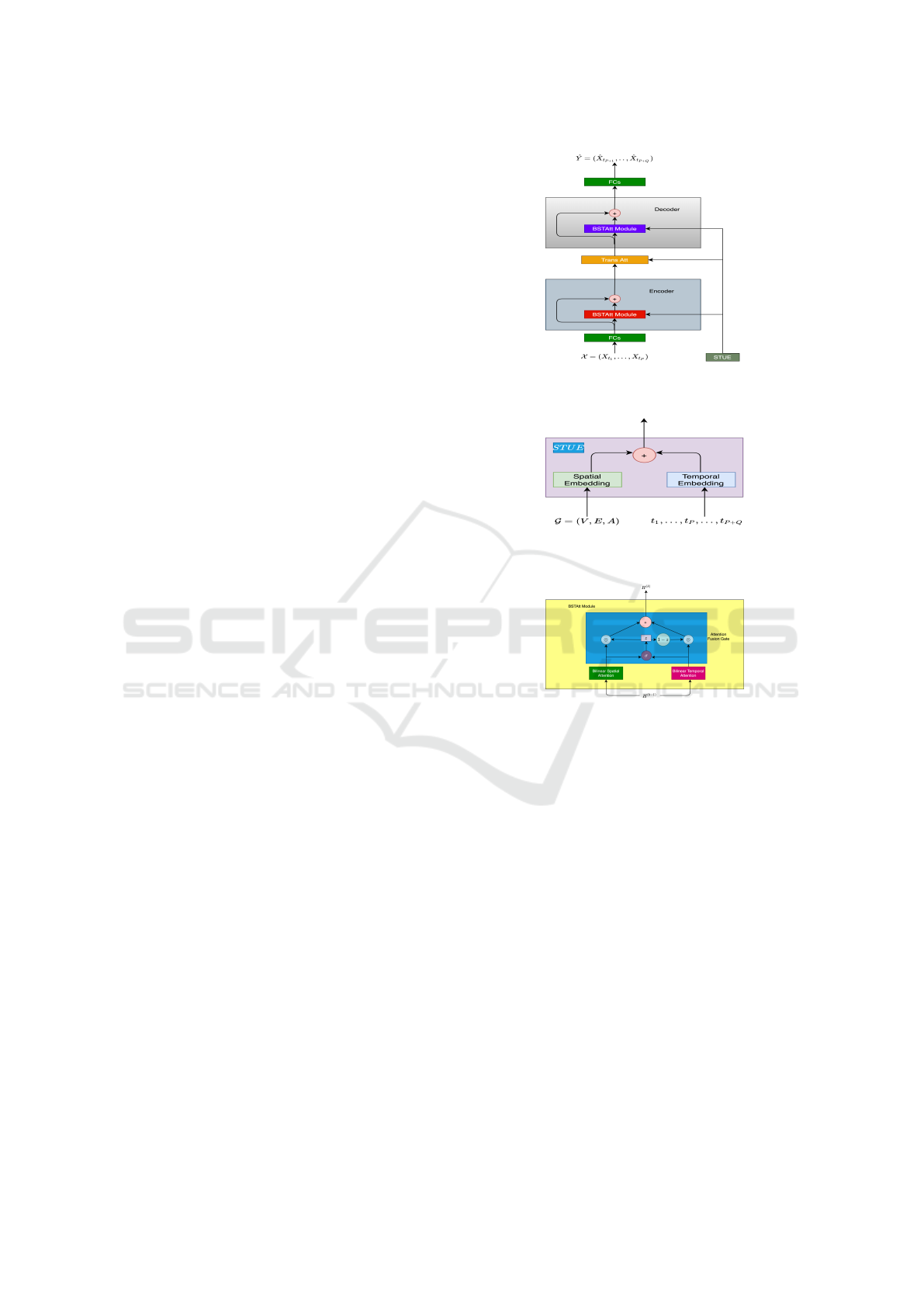
4.1 Model Overview
We show our model architecture comprehensively in
Figure 1. We adopt an end-to-end encoder-decoder
framework, for spatial embedding and temporal em-
bedding, we not only use first-order linearly weighted
features, but also use the pair-wise second-order fea-
ture interactions (Zhu et al., 2020), which can bet-
ter capture the non-linearity relationship in spatial
and temporal nodes. Both encoder and decoder con-
tain K Bilinear Spatial-Temporal Attentional blocks
(BSTAtt), each block contains three components, bi-
linear spatial attention, bilinear temporal attention
and an attention fusion gate. A transform layer is
designed between encoder and decoder layer to con-
vert the output of encoder feature to decoder. By a
spatial-temporal union embedding (STUE), we incor-
porate the graph structure and time information into
the multi-head attention mechanisms. We introduce
each module as follows in detail.
(a) The architecture of BMHA-GNN.
(b) Spatial-Temporal Union Embedding.
(c) BSTAtt Module.
Figure 1: The framework of Bilinear Multi-Head Attention
Graph Neural Network. (a) The architecture of BMHA-
GNN. (b) Spatial-Temporal Union Embedding. (c) BSTAtt
Module.
4.2 Bilinear Aggregator
In this part, we will introduce the aggregation op-
erators of GNN. Let G = (V,E,A) to represent the
spatial network, and A is the adjacency matrix, A ∈
{0,1}
N×N
, A
i j
= 1 means that an edge exists be-
tween node i and node j. N (v) = {i|A
vi
= 1}, is
a set of all nodes which has an edge with node v.
f
N (v) = v ∪N (v). We use d
v
= |N (v)| to denote the
degree of node v,
e
d
v
= d
v
+ 1.
By recursively aggregating the features from
neighbors, the spatial GNN can achieves the goal to
learn a representation vector h
v
∈ R
D
for each node v.
h
(k)
v
= AGG({h
(k−1)
i
}
i∈
f
N (v)
), (2)
where AGG represents a linear weighted sum function
Bilinear Multi-Head Attention Graph Neural Network for Traffic Prediction
35

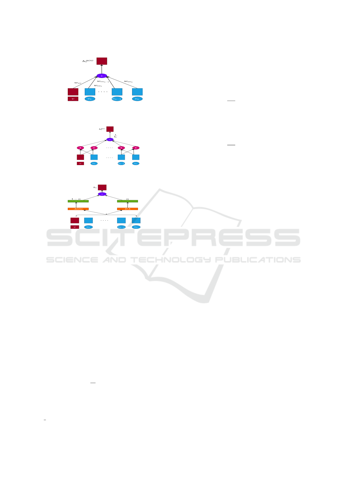
(a) AGG.
(b) BA.
(c) BGNN.
Figure 2: Aggregators in GNN; (a) is linear aggregator; (b)
is bilinear aggregator; (c) is BGNN aggregator.
of the neighborhood, h
(k−1)
i
,h
(k)
v
denotes the represen-
tation of node i, v at the k −1-th and k-th iteration,
respectively.
However, this only uses first-order nonlinear fea-
tures and does not use high-order feature combina-
tions that can better represent the target node. Al-
though a method similar to MLP can alleviate this
problem, it is implicit and inefficient (Beutel et al.,
2018).
Inspired by factorization machines (FMs) (Ren-
dle, 2010), which have been intensively used to learn
the interactions among categorical variables and is an
effective manner to model the interaction, we can de-
fine a bilinear aggregator (Zhu et al., 2020) for GNN
to model the neighbor node interactions in local struc-
ture.
BA({h
i
}
i∈
f
N (v)
) =
1
b
v
∑
i∈
f
N (v)
∑
j∈
f
N (v)&i< j
h
i
W h
j
W,
(3)
where  is element-wise product, v is the tar-
get node, i and j are node index from
f
N (v), b
v
=
1
2
e
d
v
(
e
d
v
−1) denotes the total number of interactions
for node v, W is the model parameter.
Similar to the mathematical re-formulation pro-
cess in FM (Rendle, 2010), we can transform the for-
mula (3) into the following equation:
BA({h
i
}
i∈
f
N (v)
) =
1
2b
v
∑
i∈
f
N (v)
∑
j∈
f
N (v)
s
i
s
j
−
∑
i∈
f
N (v)
s
i
s
i
!
=
1
2b
v

∑
i∈
f
N (v)
s
i

2
−
∑
i∈
f
N (v)
s
2
i
!
,
(4)
where s
i
= h
i
W ∈ R
D
. From (Zhu et al., 2020), the
bilinear aggregator is permutation invariant and the
time complexity is O(|
f
N (v)|).
Then, we can define a new graph convolution op-
erator as follows:
H
(k)
= BGNN(H
(k−1)
,A)
= (1 −α) ·AGG(H
(k−1)
,A) + α ·BA(H
(k−1)
,A),
(5)
where α is a hyperparameter to adjust the weight of
the traditional GNN aggregator and bilinear aggre-
gator, and H
(k)
is the node representation at the k-th
layer. Figure 2 illustrates three different GNN aggre-
gators.
We can also define the 2-layer BGNN model as
follows:
BGNN
2
(X,A) = (1 −α) ·GNN
2
(X,A)
+ α[(1 −β) ·BA(X,A)
+ β ·BA(X,A
(2)
)],
(6)
where
GNN
2
(H
(k)
,A) = AGG(σ(AGG(H
(k−1)
,A)), A)
represents the 2-layer GNN, σ is a non-linear activa-
tion function, β represents the strengths of bilinear in-
teraction within 1-hop neighbors and 2-hop neighbors
and A
(2)
= binarize(AA) stores the 2-hop connectivi-
ties of the graph. binarize is the operation of special-
izing non-zero elements into 1.
4.3 Spatial-temporal Union Embedding
We introduce the spatial-temporal union embedding
(STUE) in this part. Follow the node2vec approach
(Grover and Leskovec, 2016), a spatial embedding
was proposed (Zheng et al., 2020) to encode vertices
ICAART 2022 - 14th International Conference on Agents and Artificial Intelligence
36

into vectors, which can preserve the graph structure
information. By co-train the pre-learned vectors with
the whole model and feed these vectors into a fully-
connected neural network, we can obtain the spatial
embedding e
S
v
i
∈ R
D
, where v
i
∈V . However, we can
only get the static spatial embedding, which cannot
represent the road network that changes according to
time. For this reason, we also propose time embed-
ding similar to (Zheng et al., 2020), we encode the
time-of-day and day-of-week of each time step into
R
T
and R
7
by one-hot encoding, concatenate these
two into a vector of R
T +7
, and feed it into a fully-
connected neural network, we can get a vector of R
D
,
which is represented as e
T
t
j
∈R
D
, where 1 ≤ j ≤P+Q,
P stands for the historical time steps, and Q stands for
the future time steps. For vertex v
i
at time step t
j
, we
can obtain the STUE embedding by spatial embed-
ding and time embedding, that is, e
v
i
,t
j
= f (e
S
v
i
,e
S
t
j
),
f is a function. For simplicity, f can be defined as
the summation of two vectors. Thus, STUE contains
both spatial information and temporal information.
4.4 Bilinear Spatial-temporal Attention
Block
As shown in Figure 1 (c), there are three components
in the BSTAtt Block, bilinear spatial attention, bilin-
ear temporal attention and an attention fusion gate.
We represent the input of k
th
block as H
(k−1)
, h
(k−1)
v
i
,t
j
as the representation of the hidden state of vertex v
i
at time step t
j
. We denote H
(k)
S
, H
(k)
T
as the repre-
sentation of the output of bilinear spatial and bilinear
temporal attention in the k
th
block, where hs
(k)
v
i
,t
j
and
ht
(k)
v
i
,t
j
represents the hidden state of vertex v
i
at time
step t
j
, respectively. We obtain the output of k
th
block
after the attention fusion gate, denoted as H
(k)
.
4.4.1 Bilinear Spatial Attention
In order to adaptively caputure the correlations be-
tween sensors in the road network, we design a bilin-
ear spatial attention mechanism to represent the target
node embedding. For node v
i
at time step t
j
, we can
obtain a first order weighted sum from all vertices.
hs
(k)
v
i
,t
j
= AGG(h
(k−1)
v,t
j
)
=
∑
v∈V
α
v
i
,v
·h
(k−1)
v,t
j
(7)
We compute the relevance between vertex v
i
and v
by concatenate the hidden state with spatial-temporal
union embedding and adopt the scaled dot-product
approach (Vaswani et al., 2017).
s
v
i
,v
=
D
h
(k−1)
v
i
,t
j
ke
v
i
,t
j
,h
(k−1)
v,t
j
ke
v,t
j
E
√
2D
, (8)
where krepresents the concatenation operation,
h
•,•
i
represents the inner product operator. Via softmax,
s
v
i
,v
is normalized as:
α
v
i
,v
=
exp(s
v
i
,v
)
∑
v
r
∈V
exp(s
v
i
,v
r
)
.
(9)
Similar to (Zheng et al., 2020), we also extend the
spatial embedding mechanism to multi-head ones to
stabilize the learning process. L denotes the total
number of parallel attention.
s
(l)
v
i
,v
=
D
f
(l)
s,2
(h
(k−1)
v
i
,t
j
ke
v
i
,t
j
), f
(l)
s,3
(h
(k−1)
v,t
j
ke
v,t
j
)
E
√
d
,
(10)
α
(l)
v
i
,v
=
exp(s
(l)
v
i
,v
)
∑
v
r
∈V
exp(s
(l)
v
i
,v
r
)
,
(11)
hs
(k)
v
i
,t
j
= AGG(h
(k−1)
v
i
,t
j
)
=


L
l=1

∑
v∈V
α
(l)
v
i
,v
· f
(l)
s,1
(h
(k−1)
v,t
j
)

,
(12)
where f
(l)
s,1
(•), f
(l)
s,2
(•), and f
(l)
s,3
(•) denote different
non-linear projections in the l
th
attention head, and
d = D/L.
We define the spatial second-order interactions
weighted sum as follows:
hs
(k)
v
i
,t
j
= BA({h
(k−1)
v
m
,t
j
}
v
m
∈
f
N (v
i
)
)
=
1
2b
v
∑
v
m
∈
f
N (v
i
)
∑
v
n
∈
f
N (v
i
)
s
v
m
s
v
n
−
∑
v
m
∈
f
N (v
i
)
s
v
m
s
v
m
!
=
1
2b
v

∑
v
m
∈
f
N (v
i
)
s
v
m

2
−
∑
v
m
∈
f
N (v
i
)
s
2
v
m
!
,
(13)
where s
v
m
= h
(k−1)
v
m
,t
j
W ∈ R
D
, s
v
n
= h
(k−1)
v
n
,t
j
W ∈ R
D
and
b
v
=
1
2
e
d
v
(
e
d
v
−1) denotes the total number of interac-
tions for node v
i
.
Thus, the bilinear aggregator is defined beblow:
H
(k)
S
= BGNN(H
(k−1)
,A)
= (1 −α) ·AGG(H
(k−1)
,A) + α ·BA(H
(k−1)
,A),
(14)
Bilinear Multi-Head Attention Graph Neural Network for Traffic Prediction
37

where H
(k)
S
∈R
T ×N×D
stores the node representations
at the k-th layer, T = P in encoder module and T = Q
in decoder module. And α is a hyper-parameter to
adjust the traditional GNN aggregator and bilinear ag-
gregator. We can also define the 2-layer GNN model
GNN
2
(H
(k−1)
,A) = AGG(σ(AGG(H
(k−1)
,A)), A),
(15)
H
(k)
S
= BGNN
2
(H
(k−1)
,A)
= (1 −α) ·GNN
2
(H
(k−1)
,A)
+ α[(1 −β) ·BA(H
(k−1)
,A)
+ β ·BA(H
k−1
,A
(2)
)],
(16)
where A
(2)
= binarize(AA) stores the 2-hop connec-
tivities of the graph, β represents the strengths of bi-
linear interaction within 1-hop neighbors and 2-hop
neighbors and σ is a non-linear activation function.
4.4.2 Bilinear Temporal Attention
As for vertex v
i
, we define the correlation between
time step t
j
and t as follows, the process is similar
to bilinear spatial attention. The difference is that,
we only consider the time information earlier than the
target step.
u
(l)
t
j
,t
=
D
f
(l)
t,2
(h
(k−1)
v
i
,t
j
ke
v
i
,t
j
), f
(l)
t,3
(h
(k−1)
v
i
,t
ke
v
i
,t
)
E
√
d
,
(17)
β
(l)
t
j
,t
=
exp(u
(l)
t
j
,t
)
∑
t
r
∈N
t
j
exp(u
(l)
t
j
,t
r
)
,
(18)
ht
(k)
v
i
,t
j
= AGG(h
(k−1)
v
i
,t
)
=


L
l=1

∑
t∈N
t
j
β
(l)
t
j
,t
· f
(l)
t,1
(h
(k−1)
v
i
,t
)

,
(19)
where N
t
j
stands for a set of time steps before t
j
.
We define the temporal second-order interactions
weighted sum as follows:
ht
(k)
v
i
,t
j
= BA({h
(k−1)
v
i
,t
m
}
t
m
∈N
t
j
)
=
1
2b
t
∑
t
m
∈N
t
j
∑
t
n
∈N
t
j
s
t
m
s
t
n
−
∑
t
m
∈N
t
j
s
t
m
s
t
m
!
=
1
2b
t

∑
t
m
∈N
t
j
s
t
m

2
−
∑
t
m
∈N
t
j
s
2
t
m
!
,
(20)
where s
t
m
= h
(k−1)
v
i
,t
m
W ∈ R
D
, s
t
n
= h
(k−1)
v
i
,t
n
W ∈ R
D
, b
t
=
1
2
|N
t
j
|(|N
t
j
|−1) denotes the total number of interac-
tions for node t
j
and |N
t
j
| denotes the number of time
steps before t
j
.
Similar to bilinear spatial embedding, we can also
define bilinear temporal embedding.
H
(k)
T
= BGNN
2
(H
(k−1)
,A)
= (1 −α) ·GNN
2
(H
(k−1)
,A)
+ α[(1 −β) ·BA(H
(k−1)
,A)
+ β ·BA(H
(k−1)
,A
(2)
)],
(21)
where A
(2)
= binarize(AA) stores the 2-hop connec-
tivities of the graph, H
(k)
T
∈ R
T ×N×D
, T = P in en-
coder module and T = Q in decoder module. α, β
has same effect as the previous section. GNN
2
has the
same definition as equation 15.
4.4.3 Attention Fusion Gate
In this part, we design an attention fusion gate (AFG)
to adatively use bilinear spatial embedding and bilin-
ear temporal embedding representations. In the k
th
block, H
(k)
S
, H
(k)
T
denotes the output of bilinear spatial
attention and bilinear temporal attention, respectively.
They both have the shapes of R
P×N×D
in the encoder
or R
Q×N×D
in the decoder. We define the attention
fusion gate as follows:
H
(k)
= η H
(k)
S
+ (1 −η) H
(k)
T
(22)
with
η = σ(H
(k)
S
W
η,1
+ H
(k)
T
W
η,2
+ b
η
),
(23)
where W
η,1
,W
η,2
∈ R
D×D
, b
η
∈ R
D
are learnable pa-
rameters,  means the element-wise product, σ(•)
represents the sigmoid function and η denotes the
gate.
4.5 Transform Attention
Between the encoder and decoder module, we design
a transform attention layer, which can ease the er-
ror propagation effect between different time steps in
the long time horizon (Zheng et al., 2020). By Spa-
tial and Temporal Union Embedding(STUE), we can
define the relevance between the historical time step
t(t = t
1
,...,t
P
) and the prediction time step t
j
(t
j
=
t
P+1
,...,t
P+Q
) as follows:
λ
(l)
t
j
,t
=
D
f
(l)
t
s
,1
(e
v
i
,t
j
), f
(l)
t
s
,2
(e
v
i
,t)
E
√
d
(24)
ICAART 2022 - 14th International Conference on Agents and Artificial Intelligence
38

η
(l)
t
j
,t
=
exp(λ
(l)
t
j
,t
)
∑
t
P
t
s
=t
1
exp(λ
(l)
t
j
,t
s
)
(25)
by adaptively selecting relevant features from all his-
torical P time steps, the encoded traffic feature is
transformed to the decoder with the attention score
η
(l)
t
j
,t
.
h
(k)
v
i
,t
j
=


L
l=1

t
P
∑
t=t
1
η
(l)
t
j
,t
· f
(l)
t
s
,3
(h
(k−1)
v
i
,t
)

,
(26)
where f
(l)
t
s
,1
, f
(l)
t
s
,2
, f
(l)
t
s
,3
are shared learnable parameters
by all vertices and time steps.
4.6 Encoder-decoder Framework
In Figure 1, we fully demonstrate the architecture of
our model, which uses an end-to-end encoder-decoder
structure. We summarize the pipeline and tensor di-
mensions of our model in Figure 3. Firstly, we ob-
tain the historical data X ∈R
P×N×C
. After a two-layer
fully connected network, we obtain H
(0)
∈R
P×N×D
as
the input of the encoder. After K BSTAtt blocks, we
obtain the output of the encoder H
(K)
∈ R
P×N×D
. We
obtain H
(K+1)
∈ R
Q×N×D
after a transform module.
We obtain H
(2K+1)
after K BSTAtt decoder blocks
and feed it into two fully connected network, we ob-
tain the final predict value
ˆ
Y ∈ R
Q×N×C
.
4.7 Loss Function
We select mean absolute error (MAE) as our loss
function.
L(Θ) =
1
Q
t
P+Q
∑
t=t
P+1
|Y
t
−
ˆ
Y
t
|, (27)
where Θ represents all learnable parameters in
BMHA-GNN, Y
t
and
ˆ
Y
t
denote the ground truth and
predict value at time step t, respectively.
5 EXPERIMENTS
5.1 Datasets
We evaluate BMHA-GNN on two different public
traffic network datasets, METR-LA and PEMS-BAY
(Li et al., 2018). METR-LA estimates four months
of traffic velocity figures, spanning from March 1st
2012 to June 30th 2012, including 207 sensors on Los
Angeles County highways. PEMS-BAY provides five
Table 1: Details of PEMS-BAY and METR-LA.
Dataset ] Nodes ] Edges ] Time-Steps
PEMS-BAY 325 2369 52116
METR-LA 207 1515 34272
months of traffic speed figures, spanning from Jan-
uary 1st 2017 to May 31th 2017, with 325 sensors in
the BAY area. We follow the same protocols for data
pre-processing as Li et al (Li et al., 2018). Sensors’
observations are aggregated into 5-minute windows
and the data is normalized via the Z-Score method.
The details of the dataset are listed in Table 1 and the
distribution of sensors are visualized in Figure 4. Ac-
cording to some previous practices (Li et al., 2018),
we divide the dataset into training set, validation set,
and test set, with a ratio of 7:1:2. Each traffic sensor
is considered as a vertex and the node-wise graph’s
adjacency matrix is constructed by the road network
distance with the Gaussian kernel threshold (Shuman
et al., 2012). We define the adjacency matrix A simi-
lar to (Zheng et al., 2020) as follows:
A
v
x
,v
y
=



exp(−
d
2
v
x
,v
y
σ
2
),i f exp(−
d
2
v
x
,v
y
σ
2
) ≥ ε,
0 ,otherwise
(28)
where d
v
x
,v
y
is the road network distance from sensor
v
x
to v
y
, σ and ε are thresholds to control the distri-
bution and sparsity of matrix A. We set ε = 0.1 and
σ = 10 for default.
5.2 Baselines
We compare our BMHA-GNN with the following
models:
• HA: Historical Average, We use the average of
historical data in the same time period as the pre-
diction result.
• VAR (J.D., 1994): A classic time series predic-
tion model, which utilize vector auto-regression
method.
• FC-LSTM: Fully connected long short term mem-
ory network (Sutskever et al., 2014) for predic-
tions of time series.
• DCRNN: Diffusion Convolutional Recurrent
Neural Network (Li et al., 2018), which captures
both spatial and temporal dependencies among
time series using diffusion convolution and the se-
quence to sequence learning framework together
with scheduled sampling.
• ST-GCN: Spatial-Temporal Graph Convolution
Network (Yu et al., 2017), which applies
Bilinear Multi-Head Attention Graph Neural Network for Traffic Prediction
39

Figure 3: Summary of model pipeline and tensor dimensions.
Table 2: The performance of our model and baselines on different predicting intervals.
Dataset Models
15min 30min 60min
MAE RMSE MAPE MAE RMSE MAPE MAE RMSE MAPE
METR-LA
HA 4.16 7.80 13.00% 4.16 7.80 13.00% 4.16 7.80 13.00%
VAR 4.43 7.89 10.20% 5.42 9.14 12.70% 6.52 10.12 15.80%
FC-LSTM 3.44 6.31 9.60% 3.78 7.23 10.89% 4.37 8.69 13.20%
DCRNN 2.75 5.37 7.30% 3.15 6.44 8.80% 3.6 7.58 10.50%
ST-GCN 2.88 5.74 7.60% 3.46 7.24 9.60% 4.59 9.40 12.70%
Graph WaveNet 2.69 5.15 6.90% 3.07 6.22 8.40% 3.53 7.37 10.00%
MRA-BGCN 2.67 5.12 6.80% 3.06 6.17 8.30% 3.49 7.30 10.00%
GMAN 2.81 5.37 7.66% 3.10 6.30 8.48% 3.45 7.36 10.01%
FC-GAGA 2.70 5.24 7.01% 3.04 6.19 8.31% 3.45 7.19 9.88%
BMHA-GNN 2.66 5.10 6.78% 3.04 6.16 8.30% 3.43 7.10 9.85%
PEMS-BAY
HA 2.88 5.59 6.80% 2.88 5.59 6.80% 2.88 5.59 6.80%
VAR 1.74 3.16 3.60% 2.32 4.25 5.00% 2.92 5.43 6.49%
FC-LSTM 2.04 4.18 4.80% 2.20 4.54 5.20% 2.38 4.96 5.70%
DCRNN 1.38 2.95 2.90% 1.74 3.97 3.90% 2.06 4.74 4.90%
ST-GCN 1.36 2.95 2.90% 1.81 4.27 4.20% 2.48 5.68 5.80%
Graph WaveNet 1.30 2.74 2.70% 1.63 3.70 3.70% 1.95 4.52 4.60%
MRA-BGCN 1.29 2.72 2.90% 1.61 3.67 3.80% 1.91 4.46 4.60%
GMAN 1.34 2.82 2.81% 1.62 3.72 3.63% 1.86 4.32 4.31%
FC-GAGA 1.34 2.82 2.82% 1.66 3.75 3.71% 1.93 4.40 4.48%
BMHA-GNN 1.28 2.71 2.70% 1.60 3.67 3.60% 1.82 4.30 4.28%
(a) (b)
Figure 4: Sensor distribution of the PEMS-BAY and
METR-LA dataset. (a) PEMS-BAY, (b) METR-LA.
purely convolutional structures to extract spatial-
temporal features simultaneously.
• Graph WaveNet: Graph WaveNet for Deep
Spatial-Temporal Graph Modeling (Wu et al.,
2019), which constructs a self-adaptive adjacency
matrix to capture the hidden spatial dependencies
and proposes a new graph convolution with di-
lated casual convolution.
• MRA-BGCN: Multi-Range Attentive Bicompo-
nent Graph Convolution Network (Chen et al.,
2019), which proposes the bicomponent graph
convolution to explicitly model the corrections of
both nodes and edges.
• GMAN: A Graph Multi-Attention Network
(Zheng et al., 2020), which proposes spatial-
temporal attention mechanisms to model the dy-
namic spatial and non-linear temporal correla-
tions.
• FC-GAGA: Fully Connected Gated Graph Ar-
chitecture (Oreshkin et al., 2020), which uses
hard graph gating mechanism and fully connected
time-series forecasting architecture.
5.3 Experimental Results
5.3.1 Experiments Settings
Firstly, we recall the definition of our task, f :
R
P×N×C
→R
Q×N×C
We are given the historical traffic
data of the past hour and predict the traffic data of the
next hour, i.e., P = Q = 12.
In our experiment, we set the number of BSTAtt
Module K to 3, and the dimension of vertex D to 64.
We set the number of multi-head L to 8 and the out-
put dimension of each attention head d is 8. We set
the Bilinear aggregator parameters α = 0.3 for bilin-
ear spatial attention, and α = 0.2 for bilinear tem-
poral attention. We set β = 0.7 to control the one-
hop and two-hop neighbors. We set the max epoch
to 500, if the validation loss does not decrease in the
last 20 epochs, it will be terminated early. We use the
AdamOptimizer (Kingma and Ba, 2014) to minimize
loss, and the learning rate is set to 0.001.
ICAART 2022 - 14th International Conference on Agents and Artificial Intelligence
40

In order to show our experimental results more ob-
jectively, we ran each experiment 10 times through
different initialization seeds and took the average
value to represent the final result. At the same time,
the confidence p value is 0, which objectively shows
the superiority of our experimental results. We will
also open source code in the future for everyone to
reproduce.
5.3.2 Evaluate Metrics
We adopt the three most common traffic prediction
indicators to evaluate our model: (1) Mean Absolute
Error (MAE), (2) Root Mean Squared Error (RMSE),
and (3) Mean Absolute Percentage Error (MAPE).
5.3.3 Performance Comparison
Table 2 shows the performance of our BMHA-GNN
model and nine baseline models on two datasets,
METR-LA, PEMS-BAY (Li et al., 2018). We divided
the 1h prediction results into short time (15min),
medium time (30min), and long time (1h). We can
see from Table 2 that our model achieves the state-of-
the-art in most scenarios.
Compare with these baseline models, we observe
the following phenomena: (1) The performance of
GNN-based models will be better than other models,
because GNNs can better capture the dependency be-
tween spatial and temporal. (2) The use of bilinear
aggregator in spatial embedding and temporal embed-
ding can learn higher-order information and combina-
tion features. We believe that if two nodes appear at
the same time, it will be a very strong signal for the
current target node.
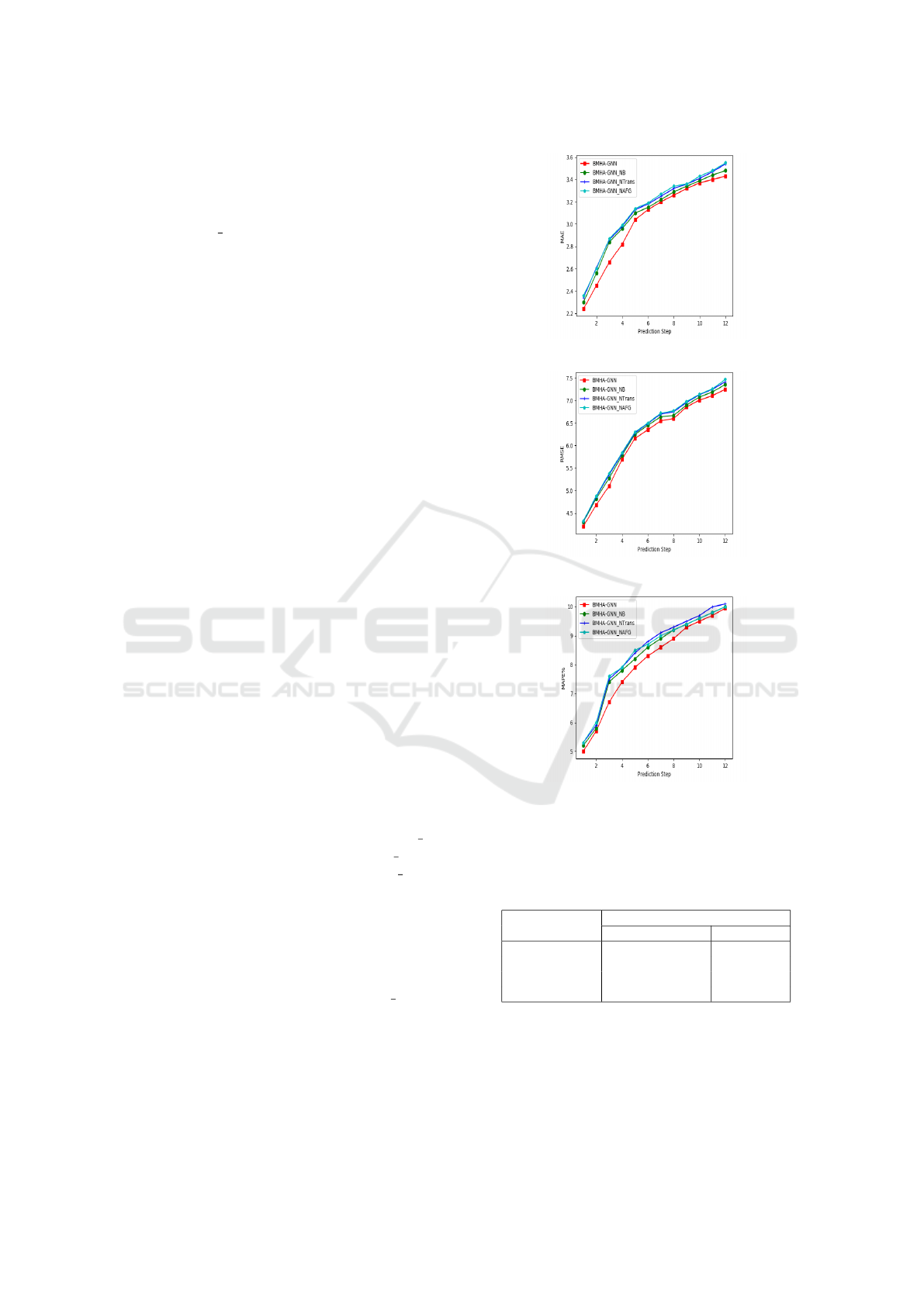
5.3.4 Ablation Study
To verify the effect of each module, we make sev-
eral variants for BMHA-GNN, BMHA-GNN NB
(without Bilinear aggregator), BMHA-GNN NTrans
(without Transform Attention), BMHA-GNN NAFG
(without Attention Fusion Gate). As we all know,
the dataset of METR-LA is more complicated and it
is more difficult to estimate. Therefore the ablation
study experiments will use this dataset.
Figure 5 shows the three indicators on the METR-
LA dataset. From it, we can see that the performance
of BMHA-GNN is better than BMHA-GNN NB sig-
nificantly, which proves that the bilinear aggregator
we propose is effective.
5.3.5 Time Cost
We train and inference on a GPU machine, Tesla
V100-SXM2-32GB. We list the time-consuming sit-
(a)
(b)
(c)
Figure 5: Performance of each prediction step in METR-
LA with Three variants. (a) The metrics of MAE, (b) The
metrics of RMSE, and (c) The metrics of MAPE.
Table 3: Time-consuming of different models on PEMS-
BAY.
Models
Computation-Time
Training(s/epoch) Inference(s)
DCRNN 689.92 132.45
GMAN 245.87 15.34
Graph WaveNet 203.18 9.87
BMHA-GNN 359.42 19.22
uation of several models, including training and in-
ference process in Table 3. As shown in Table 3,
DCRNN takes the highest computation time because
it requires iterative calculation to generate 12 steps
prediction score. Our model takes higher time than
GMAN and Graph WaveNet. The reason is that we
Bilinear Multi-Head Attention Graph Neural Network for Traffic Prediction
41

add the calculation logic of bilinear, and the parame-
ters of the model have also been relatively increased.
However, compared to the improvement of the model
performance, we believe that this conversion is cost-
effective.
6 CONCLUSION
We propose an end-to-end Bilinear Multi-Head At-
tention Graph Neural Network for Traffic Prediction,
which not only utilize the linear weighted neighbor
nodes to represent the target spatial and temporal
node, but also use the bilinear aggregator in spatial
and temporal representations. Extensive experiments
are carried out on two real-word traffic datasets, and
the results show that our proposed model achieves the
state-of-the-art performance in most scenes. For fu-
ture work, we will consider encoding high-order in-
teractions among multiple neighbors to represent the
target node and apply our model to other related ap-
plications.
ACKNOWLEDGEMENTS
This work was supported by the National Key R&D
Program of China under Grant No.2018AAA0101204
and No.2018AAA0101200. Kai Han is the corre-
sponding author.
REFERENCES
Atwood, J. and Towsley, D. (2015). Search-convolutional
neural networks. volume abs/1511.02136.
Beutel, A., Covington, P., Jain, S., Xu, C., Li, J., Gatto, V.,
and Chi, E. H. (2018). Latent cross: Making use of
context in recurrent recommender systems. In WSDM,
pages pages 46–54.
Bruna, J., Zaremba, W., Szlam, A., and Lecun, Y. (2014).
Spectral networks and locally connected networks on
graphs. In International Conference on Learning Rep-
resentations (ICLR2014), CBLS, April 2014.
Chen, W., Chen, L., Xie, Y., Cao, W., Gao, Y., and Feng,
X. (2019). Multi-range attentive bicomponent graph
convolutional network for traffic forecasting. volume
abs/1911.12093.
Chun-Hsin Wu, Jan-Ming Ho, and Lee, D. T. (2004).
Travel-time prediction with support vector regression.
volume 5, pages 276–281.
Chung, J., G
¨
ulc¸ehre, C¸ ., Cho, K., and Bengio, Y. (2014).
Empirical evaluation of gated recurrent neural net-
works on sequence modeling. volume abs/1412.3555.
D., N., N., N., Y., G., , and H., K. (2005). Univariate short-
term prediction of road travel times. In In Proceed-
ings of IEEE Intelligent Transportation Systems Con-
ference, pages 1074–1079.
Grover, A. and Leskovec, J. (2016). node2vec:
Scalable feature learning for networks. volume
abs/1607.00653.
J.D., H. (1994). Time series analysis. volume Volume 2,
pages 690–696.
Kingma, D. and Ba, J. (2014). Adam: A method for
stochastic optimization.
Li, Y., Yu, R., Shahabi, C., and Liu, Y. (2018). Diffusion
convolutional recurrent neural network: Data-driven
traffic forecasting. In International Conference on
Learning Representations (ICLR ’18).
Ma, X., Dai, Z., He, Z., and Wang, Y. (2017). Learning
traffic as images: A deep convolution neural network
for large-scale transportation network speed predic-
tion. volume abs/1701.04245.
Nikovski, D., Nishiuma, N., Goto, Y., and Kumazawa, H.
(2005). Univariate short-term prediction of road travel
times. In Proceedings. 2005 IEEE Intelligent Trans-
portation Systems, 2005., pages 1074–1079.
Oreshkin, B. N., Amini, A., Coyle, L., and Coates, M. J.
(2020). Fc-gaga: Fully connected gated graph archi-
tecture for spatio-temporal traffic forecasting.
Q., Z., J., C., G., M., S., X., and C., P. (2020). Spatio-
temporal graph structure learning for traffic forecast-
ing. In Proceedings of the AAAI Conference on Artifi-
cial Intelligence, pages 1177–1185.
Rendle, S. (2010). Factorization machines. In 2010 IEEE
International Conference on Data Mining, pages 995–
1000.
S., G., Y., L., N., F., C., S., and H., W. (2019). Attention
based spatial-temporal graph convolutional networks
for traffic flow forecasting. pages 922–929.
Shuman, D. I., Narang, S. K., Frossard, P., Ortega, A.,
and Vandergheynst, P. (2012). Signal processing on
graphs: Extending high-dimensional data analysis to
networks and other irregular data domains. volume
abs/1211.0053.
S.I.J., C. and C.M., K. (2003). Dynamic travel time pre-
diction with real-time and historic data. In Journal of
Transportation Engineering 129(6), pages 608–616.
Song, C., Lin, Y., Guo, S., and Wan, H. (2020). Spatial-
temporal synchronous graph convolutional networks:
A new framework for spatial-temporal network data
forecasting. volume 34, pages 914–921.
Sutskever, I., Vinyals, O., and Le, Q. V. (2014). Sequence to
sequence learning with neural networks. In Proceed-
ings of the 27th International Conference on Neural
Information Processing Systems - Volume 2, NIPS’14,
page 3104–3112, Cambridge, MA, USA. MIT Press.
Vaswani, A., Shazeer, N., Parmar, N., Uszkoreit, J., Jones,
L., Gomez, A. N., Kaiser, u., and Polosukhin, I.
(2017). Attention is all you need. In Proceedings of
the 31st International Conference on Neural Informa-
tion Processing Systems, NIPS’17, page 6000–6010,
Red Hook, NY, USA. Curran Associates Inc.
ICAART 2022 - 14th International Conference on Agents and Artificial Intelligence
42

Wu, Z., Pan, S., Long, G., Jiang, J., and Zhang, C. (2019).
Graph wavenet for deep spatial-temporal graph mod-
eling. volume abs/1906.00121.
Xu, K., Hu, W., Leskovec, J., and Jegelka, S. (2019). How
powerful are graph neural networks? In International
Conference on Learning Representations.
Xuan, S., Hiroshi, K., and Ryosuke, S. (2016). Deep-
transport: Prediction and simulation of human mobil-
ity and transportation mode at a citywide level. In
Proceedings of the Twenty-Fifth International Joint
Conference on Artificial Intelligence, IJCAI’16, page
2618–2624. AAAI Press.
Yao, H., Tang, X., Wei, H., Zheng, G., Yu, Y., and Li, Z.
(2018a). Modeling spatial-temporal dynamics for traf-
fic prediction. volume abs/1803.01254.
Yao, H., Wu, F., Ke, J., Tang, X., Jia, Y., Lu, S., Gong, P.,
Ye, J., and Li, Z. (2018b). Deep multi-view spatial-
temporal network for taxi demand prediction. volume
abs/1802.08714.
Yu, B., Yin, H., and Zhu, Z. (2017). Spatio-temporal graph
convolutional neural network: A deep learning frame-
work for traffic forecasting. volume abs/1709.04875.
Zheng, C., Fan, X., Wang, C., and Qi, J. (2020). Gman: A
graph multi-attention network for traffic prediction. In
AAAI, pages 1234–1241.
Zheng, Z. and Su, D. (2014). Short-term traffic volume fore-
casting: A k-nearest neighbor approach enhanced by
constrained linearly sewing principle component al-
gorithm. volume 43, pages 143–157. Special Issue on
Short-term Traffic Flow Forecasting.
Zhu, H., Feng, F., He, X., Wang, X., Li, Y., Zheng, K., and
Zhang, Y. (2020). Bilinear graph neural network with
node interactions.
Bilinear Multi-Head Attention Graph Neural Network for Traffic Prediction
43