
Towards Multi-agent Reinforcement Learning using
Quantum Boltzmann Machines
Tobias M
¨
uller, Christoph Roch, Kyrill Schmid and Philipp Altmann
Mobile and Distributed Systems Group, LMU Munich, Germany
Keywords:
Multi-agent, Reinforcement Learning, D-Wave, Boltzmann Machines, Quantum Annealing, Quantum
Artificial Intelligence.
Abstract:
Reinforcement learning has driven impressive advances in machine learning. Simultaneously, quantum-
enhanced machine learning algorithms using quantum annealing underlie heavy developments. Recently, a
multi-agent reinforcement learning (MARL) architecture combining both paradigms has been proposed. This
novel algorithm, which utilizes Quantum Boltzmann Machines (QBMs) for Q-value approximation has out-
performed regular deep reinforcement learning in terms of time-steps needed to converge. However, this
algorithm was restricted to single-agent and small 2x2 multi-agent grid domains. In this work, we propose
an extension to the original concept in order to solve more challenging problems. Similar to classic DQNs,
we add an experience replay buffer and use different networks for approximating the target and policy values.
The experimental results show that learning becomes more stable and enables agents to find optimal policies
in grid-domains with higher complexity. Additionally, we assess how parameter sharing influences the agents’
behavior in multi-agent domains. Quantum sampling proves to be a promising method for reinforcement
learning tasks, but is currently limited by the Quantum Processing Unit (QPU) size and therefore by the size
of the input and Boltzmann machine.
1 INTRODUCTION
Recently, adiabatic quantum computing has proven
to be a useful extension to machine learning tasks
(Benedetti et al., 2018; Biamonte et al., 2017; Li et al.,
2018; Neukart et al., 2017a). Especially hard com-
putational tasks with high data volume and dimen-
sionality have benefitted from the possibility of using
quantum devices with manufactured spins to speed-
up computational bottlenecks (Neven et al., 2008;
Rebentrost et al., 2014; Wiebe et al., 2012).
One specific type of machine learning is Rein-
forcement Learning (RL), where an interacting entity,
called agent, aims to learn an optimal state-action pol-
icy through trial and error (Sutton and Barto, 2018).
Reinforcement Learning has gained the public atten-
tion by defeating the 9-dan Go grandmaster Lee Sedol
(Silver et al., 2016), which has been thought to be
impossible for a machine. In the latest years, re-
inforcement learning has seen many improvements,
gained a large variety of application fields like eco-
nomics (Charpentier et al., 2020), autonomous driv-
ing (Kiran et al., 2020), biology (Mahmud et al.,
2018) and even achieved superhuman performance
in chip design (Mirhoseini et al., 2020). Reinforce-
ment Learning has only seen quantum speed-ups for
specials models (Levit et al., 2017; Neukart et al.,
2017a; Neukart et al., 2017b; Paparo et al., 2014).
Especially multi-agent domains have rarely been re-
searched (Neumann et al., 2020).
Real-world reinforcement learning frameworks
predominantly use deep neural networks (DNNs) as
function approximators. Since DNNs are powerful -
see the latest prominent example AlphaFold2 (Jumper
et al., 2020) - and can be run efficiently for large
datasets on classical computers, deep reinforcement
learning is able to tackle complex problems in large
data spaces. Hence, there was little need for improve-
ments.
However, since recent work has proved speed-
ups for classical RL by leveraging quantum comput-
ing (Levit et al., 2017; Neumann et al., 2020) and
the application field gets more and more complex,
it could be beneficial to explore quantum RL algo-
rithms. These inspiring studies considered Boltzmann
machines (Ackley et al., 1985) as function approxi-
mator - instead of traditionally used DNNs. Boltz-
mann machines are stochastic neural networks, which
Müller, T., Roch, C., Schmid, K. and Altmann, P.
Towards Multi-agent Reinforcement Learning using Quantum Boltzmann Machines.
DOI: 10.5220/0010762100003116
In Proceedings of the 14th International Conference on Agents and Artificial Intelligence (ICAART 2022) - Volume 1, pages 121-130
ISBN: 978-989-758-547-0; ISSN: 2184-433X
Copyright
c
2022 by SCITEPRESS – Science and Technology Publications, Lda. All rights reserved
121

are mainly avoided due to the fact, that their training
times are exponential to the input size. Since find-
ing the energy minimum of Boltzmann machines can
be formulated as a ”Quadratic Unconstrained Binary
Optimization” (QUBO) problem, simulated anneal-
ing respectively quantum annealing is well suited to
accelerate training time.
Nevertheless, the combination of RL and Boltz-
mann machines using (simulated) quantum annealing
only worked properly for small single-agent environ-
ments and reached its limit at a simple 3 × 3 multi-
agent domain. This work proposes an architecture in-
spired by DQNs (Mnih et al., 2015) to enable more
complex domains and stabilize learning by using ex-
perience replay buffer and separating policy and tar-
get networks. We thoroughly evaluate the effects of
these augmentations on learning.
Lately, an inspiring novel method to speed-up
quantum reinforcement learning for large state and
action spaces by proposing a combination of reg-
ular NNs and DBMs/QBMs, namely Deep Energy
Based Networks (DEBNs) was proposed (Jerbi et al.,
2020). More specifically, these architectures are con-
structed with an input layer consisting of action and
state units, which are connected with the first hidden
layer through directed weights. This is followed by
a single undirected stochastic layer. The remaining
layers are linked with directed deterministic connec-
tions. Lastly, a final output layer returns the negative
free energy −F(s, a).
In contrast to QBMs, DEBNs therefore only com-
prise one stochastic layer, return an output similar to
traditional deep neural networks and can be trained
through backpropagation. DEBNs also use an expe-
rience replay buffer and separate the policy and tar-
get network. Additionally, they allow to trade off
learning performance for efficiency of computation.
Jerbi et al. briefly stated, that QBMs are applica-
ble. Unfortunately, no numerical results were given
for purely stochastic, energy-based QBM agents or
domains with multiple agents. We aim to build on
this.
Summarized, our contribution is three-fold:
• We provide a Quantum Reinforcement Learn-
ing (Q-RL) framework, which stabilizes learning
leading to more optimal policies
• Based on single- and multi-agent domains, we
provide a thorough evaluation on the effects of an
Experience Replay Buffer and an additional Tar-
get Network compared to traditional QBM agents
• Additionally, we demonstrate and discuss limita-
tions to the concept
We first describe the preliminaries about rein-
forcement learning and quantum Boltzmann ma-
chines underlying the proposed architectures. After-
wards, the state-of-the-art algorithm and extensions
made to it will be explained. We test and evaluate the
approach and finally discuss restrictions and potential
grounds for future work.
2 PRELIMINARIES
This chapter describes the basics needed to under-
stand our proposed architecture. First, reinforcement
learning and the underlying Markov Decision Process
will be explained followed by Boltzmann Machines
and the process of quantum annealing.
2.1 Reinforcement Learning
We first describe Markov Decision Processes as the
underlying problem formulation which is followed by
an introduction to reinforcement learning in general.
The subsequent sections specify independent and co-
operative multi-agent reinforcement learning.
Markov Decision Processes. The problem formu-
lation is based on the notion of Markov Decision Pro-
cesses (MDP) (Puterman, 1994). MDPs are a class
of sequential decision processes and described via the
tuple M = hS, A, P, Ri, where
• S is a finite set of states and s
t
∈ S the state of the
MDP at time step t.
• A is the set of actions and a
t
∈ A the action the
MDP takes at time step t.
• P(s
t+1
|s
t
, a
t
) is the probability transition function.
It describes the transition that occurs when action
a
t
is executed in state s
t
. The resulting state s
t+1
is chosen according to P.
• R(s
t
, a
t
) is the reward, when the MDP takes action
a
t
in state s
t
. We assume R(s
t
, a
t
) ∈ R
Consequently, the cost and transition function
only depend on the current state and action of the
system. Eventually, the MDP should find a policy
π : S → A in the space of all possible policies Π, which
maximizes the return G
t
at state s
t
over an infinite
horizon via:
G
t
=
∞
∑
k=0
γ
k
· R(s
t+k
, a
t+k
), (1)
with γ ∈ [0, 1] as the discount factor. This policy is
called the optimal policy π.
ICAART 2022 - 14th International Conference on Agents and Artificial Intelligence
122
Reinforcement Learning. Model-free reinforce-
ment learning (Strehl et al., 2006) is considered to
search the policy space Π in order to find the opti-
mal policy π
∗
. The interacting reinforcement learn-
ing agent executes an action a
t
for every time step
t ∈ [1, ..] in the MDP environment. In model-free al-
gorithms, the agent acts without any knowledge of the
environment and the algorithm only keeps informa-
tion of the value-function. Therefore, the agent knows
its current state s
t
and the action space A, but neither
the reward nor the next state s
t+1
of any action a
t
in
any state s
t
.
Consequently, the agent needs to learn from delayed
rewards without having a model of the environment.
A popular value-based approach to solve this problem
is Q-learning (Peng and Williams, 1994). In this ap-
proach, the action-value function Q
π
: SxA → R, π ∈ Π
describes the accumulated reward Q
π
(s
t
, a
t
) for an ac-
tion a
t
in state s
t
. The optimal Q-learning function Q
∗
is approximated by starting from an initial guess for
Q and updating the function via:
Q(s
t
, a
t
) ← Q(s
t
, a
t
) + α[r
t
+ γ max
a
Q(s
t+1
, a) − Q(s
t
, a
t
)]
(2)
The learned Q-function will eventually converge
to Q
∗
, which then implies an optimal policy. In the
traditional experiments a deep neural network is used
as a parameterized function approximator to calculate
the optimal action for a given state.
Independent Multi-agent Learning. When mul-
tiple agents interact with the environment, A fully
cooperative multi-agent task can be described as a
stochastic game G, defined as in (Foerster et al., 2017)
via the tuple G = hS, A, P, R, Z, O, n, γi, where:
• S is a finite set of states. At each time step t, the
environment has a true state s
t
∈ S.
• A is the set of actions. At each time step t each
agent ag simultaneously chooses an action a
ag
∈
A, forming a joint action a ∈ A ≡ A
n
.
• P(s
t+1
|s
t
, a
t
) is the probability transition function
as previously defined.
• R(s
t
, a
t
) is the reward as previously defined. All
agents share the same reward function.
• Z is a set of observations of a partially or fully
observable environment.
• O(s, ag) is the observation function. Each agent
draws observations z ∈ Z according to O(s, ag).
• n is the number of agents identified by ag ∈ AG ≡
{1, ..., n}.
• γ ∈ [0, 1) is the discount factor.
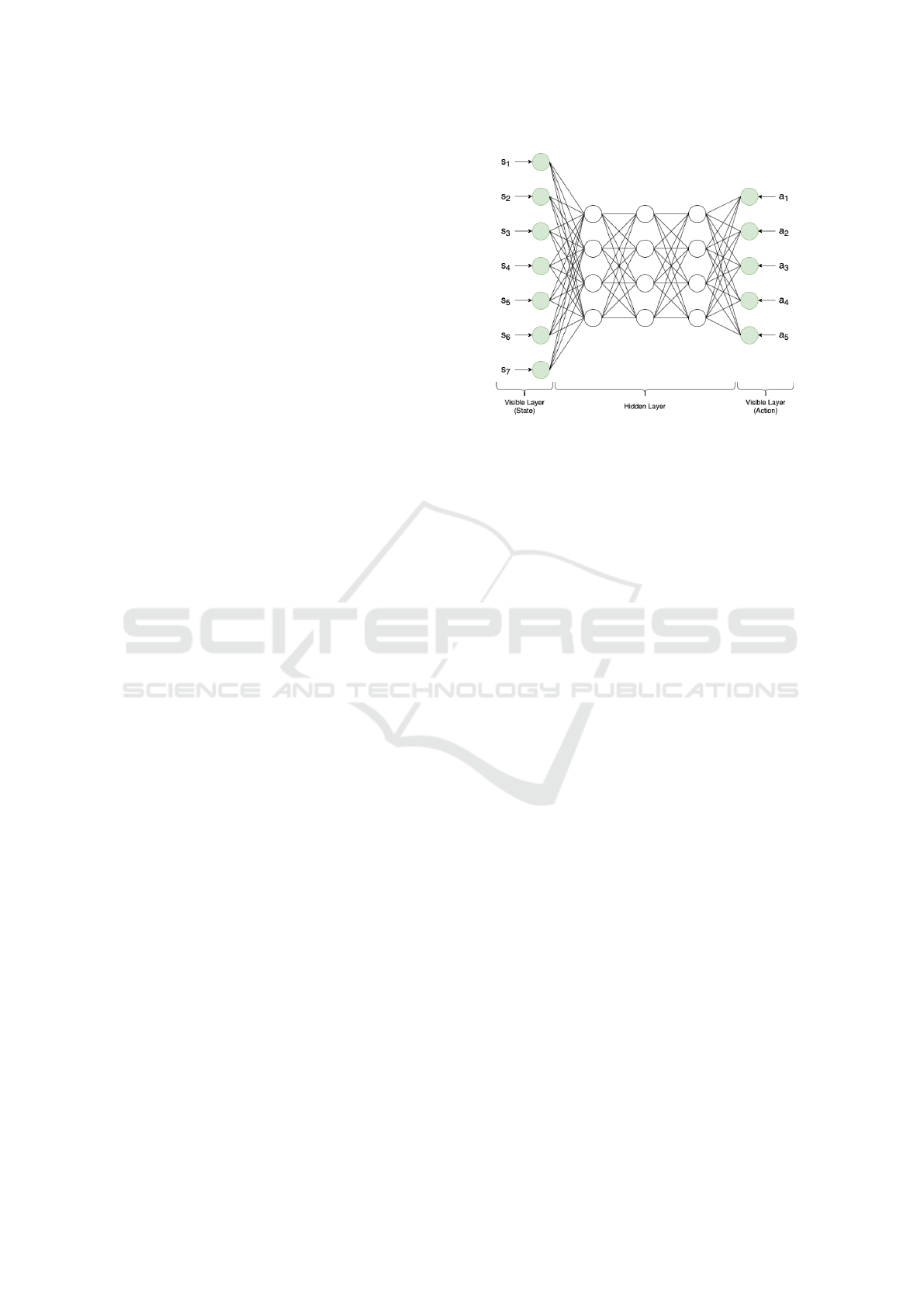
Figure 1: A Deep Quantum Boltzmann Machine with seven
input state neurons and five input action neurons. The QBM
additionally consists of three hidden layers with four neu-
rons each. The state and action are given as fixed input
and the configuration of the hidden neurons are sampled via
(simulated) quantum annealing. The weights between two
neurons are updated in the Q-learning step as described in
section 3.
In independent multi-agent learning algorithms, each
agent learns from its own action-observation history
and is trained independently. This means, every agent
simultaneously learns its own Q-function (Tan, 1993).
2.2 Boltzmann Machines
The structure of a Boltzmann machine (BM) (Ack-
ley et al., 1985) is similar to Hopfield networks and
can be described as a stochastic energy-based neural
network. A traditional BM consists of a set of visi-
ble nodes V and a set of hidden nodes H, where ev-
ery node represents a binary random variable. The
binary nodes are connected through real-valued, bidi-
rected, weighted edges of the underlying undirected
graph. The global energy configuration is generally
given by the energy level of Hopfield networks. Since
clamped BMs fix the assignment of the visible binary
variables, these nodes are removed from the under-
lying graph and contribute as constant coefficients to
the associated energy. Therefore the formula, which
we aim to minimize, is given as the energy level of
Hopfield networks with constant visible nodes:
E(h) = −
∑
i
w
ii
v
i
−
∑
j
w
j j
h
j
−
∑
i
∑
j
v
i
w
i j
h
j
, (3)
with v
i
as the visible nodes, h
j
as the hidden nodes
and weights w.
For this work, we implemented a Deep Boltzmann
Machine (DBM) as trainable state-action approxima-
tor, which is constructed with multiple hidden layers,
Towards Multi-agent Reinforcement Learning using Quantum Boltzmann Machines
123

one visible input layer for the state and one visible ac-
tion input layer. Finally, we modified the DBM to get
a Quantum Boltzmann Machine (QBM), where qubits
are associated to each node of the network instead of
random binary variables (Crawford et al., 2019; Neu-
mann et al., 2020; Levit et al., 2017). A visualization
of a QBM for seven state neurons and five input action
neurons can be seen in figure 1. For any QBM with
v ∈ V and h ∈ H, the energy function is described by
the quantum Hamiltonian H
v
:
H
v
= −
∑
v,h
w
vh
vσ
z
h
−
∑
v,v
0
w
vv
0
vv
0
−
∑
h,h
0
w
hh
0
σ
z
h
σ
z
h
0
− Γ
∑
h
σ
x
h
(4)
Furthermore, Γ is the annealing parameter, while
σ
z
i
and σx
i
are spin-values of node i in the z− and
x− direction. Because measuring the state of one
direction destroys the state of the other, we follow
the architecture of Neumann et al. (2020) (Neumann
et al., 2020) and replace all σ
x
i
by σ
z
by using replica
stacking based on the Suzuki-Trotter expansion of the
Hamiltonian H
v
. The BM is replicated r times in to-
tal and connections between corresponding nodes in
adjacent replicas are added. By this, we obtain a new
effective Hamiltonian H
e f f
v=(s,a)
in its clamped version
given by:
H
e f f
v=(s,a)
= −
∑
h∈H
h−s ad j
r
∑
k=1
w
sh
r
σ
h,k
−
∑
h∈H
h−a ad j
r
∑
k=1
w
ah
r
σ
h,k
−
∑
(h,h
0
)⊆H
r
∑
k=1
w
hh
0
r
σ
h,k
σ
h
0
,k
− Γ
∑
h∈H
r
∑
k=0
σ
h,k
σ
h,k+1
(5)
For each evaluation of the Hamiltonian, we get a
spin configuration
ˆ
h. After n
reads
reads for a fixed
combination of s and a, we get a multi-set
ˆ
h
s,a
=
{
ˆ
h
1
, ...,
ˆ
h
n
reads
}. We average over this multi-set to gain
a single spin configuration C
ˆ
h
s,a
, which will be used
for updating the network. If a node is +1 or −1 de-
pends on the global energy configuration:
p
node i=1
=
1
1 + exp(−
∆E
i
T
)
, (6)
with T as the current temperature.
Since the structure of Boltzmann Machines are
inherent to Ising models, we sample spin values
from the Boltzmann distribution by using simulated
quantum annealing, which simulates the effect of
transverse-field Ising model by slowly reducing the
temperature or strength of the transverse field at finite
temperature to the desired target value (Levit et al.,
2017). As proven in (Morita and Nishimori, 2008),
spin system defined by simulated quantum annealing
converges to quantum Hamiltonian. Therefore it is
straightforward to use simulated quantum annealing
(SQA) to find a spin configuration for h ∈ H - given
s ∈ S - which minimizes the free energy.
3 QUANTUM REINFORCEMENT
LEARNING
Recently, quantum reinforcement learning algorithms
(QRL) using boltzmann machines and quantum an-
nealing of single agent (Crawford et al., 2019) and
multi-agent domains (Neumann et al., 2020) for learn-
ing grid-traversal policies have been proposed. Al-
though, these architectures were able to learn opti-
mal policies in less time steps compared to classic
deep reinforcement learners (DRL), they could only
be applied to single-agent or small multi-agent do-
mains. Unfortunately, already 3 × 3 domains with 2
agents could not be solved optimally (Neumann et al.,
2020). QRL seems to be unstable for more complex
domains. We intuitively assume that BMs underlie
similar instability problems as traditional neural net-
works. Hence, by correlations present in the sequence
of observations and how small updates to the Q-values
change the policy, data distribution and therefore the
correlations between free energy F(s
n
, a
n
) and target
energy F(s
n+1
, a
n+1
). Inspired by Deep Q-Networks
(Mnih et al., 2015), we propose to enhance the state-
of-the-art architecture as described in section 3.1 by
adding an experience replay buffer (see section 3.2)
to randomize over transitions and by separating the
network calculating the policy and the network ap-
proximating the target value (see section 3.3) in order
to reduce correlations with the target.
3.1 State of the Art
Traditionally, single-agent reinforcement learning us-
ing quantum annealing and QBMs is an adaption
of Sallans and Hintons (2004) (Sallans and Hinton,
2004) RBM RL algorithm and structured as follows:
Initialization. The weights of the QBM are initial-
ized by setting the weights using Gaussian zero-mean
values with a standard deviation of 1.00. The topol-
ogy of the hidden layers is set beforehand.
Policy. At the beginning of each episode, every
agent is set randomly onto the grid and receives its
ICAART 2022 - 14th International Conference on Agents and Artificial Intelligence
124

corresponding observation. At each time step t, ev-
ery agent i independently chooses an action a
i
t
accord-
ing to its policy π
i
t
. To enable exploration, we imple-
mented an ε-greedy policy, where the agent acts ran-
dom with probability ε, which decreases by ε
decay
=
0.0008 with each training step until ε
min
= 0.01 is
reached. When the agent follows its learned policy,
we sweep across all possible actions and choose the
action which maximizes the Q-value for state s
i
t
. The
Q-function of state s and action a is defined as the
corresponding negative free-energy −F:
Q(s, a) ≈ −F(s, a) = −F(s, a;w), (7)
with w as the vector of weights of a QBM and F(s, a)
as:
F(s, a) = hH
e f f
v=(s,a)
i −
1
β
P(s
t+1
|s
t
, a
t
)logP(s
t+1
|s
t
, a
t
)
(8)
Summarized, the agent acts via:
π =
random, i f p ≥ ε
argmax Q(s, a), i f p < ε
(9)
for a ∈ A and random variable p.
Weight Update. The environment returns a reward
r
i
t+1
and second state s
i
t+1
← a
i
t
(s
i
t
) for each agent i.
Based on this transition, the QBM is trained. The
used update rules are an adaption of the state-action-
reward-state-action (SARSA) rule by Rummery et al.
(1994) (Rummery and Niranjan, 1994) with negative
free energy instead of Q-values (Levit et al., 2017)
defined as:
∆w
vh
= µ(r
n
(s
n
, a
n
) − γF(s
n+1
, a
n+1
)
+F(s
n
, a
n
))vhσ
z
h
i
(10)
∆w
hh
0
= µ(r
n
(s
n
, a
n
) − γF(s
n+1
, a
n+1
)
+F(s
n
, a
n
))vhσ
z
h
σ
z
h
0
i,
(11)
with γ as the discount factor and µ as the learning
rate. The free energy and configurations of the hid-
den neurons are gained by applying simulated quan-
tum annealing respectively quantum annealing to the
formulation of the effective Hamiltonian H
e f f
v=(s,a)
as
described in the previous section. At each episode,
this process is repeated for a defined number of steps
or until the episode ends.
3.2 Experience Replay Buffer
The first extension is a biologically inspired mech-
anism named experience replay (Mcclelland et al.,
1995; O’Neill et al., 2010). O’Neill et al. (2010)
found, that the human brain stabilizes memory traces
from short- to long-term memory by replaying mem-
ories during sleep and rest. The reactivation of brain-
wide memory traces could underlie memory consoli-
dation. Similar to the human brain, experience replay
buffers used in deep Q-networks (DQN) store experi-
enced transitions and provides randomized data dur-
ing updating neural connections. Hence, correlations
of observation sequences are removed and changes in
the data distribution are smoothed. Furthermore, due
to the random choice of training samples, one transi-
tion can be used multiple times to consolidate experi-
ences.
To enable experience replay, at each time step t we
store the each agents’ experience e
t
= (s
t
, a
t
, r
t
, s
t+1
)
in a data set D
t
= (e
1
, ..., e
t
). For every training
step, we randomly sample mini-batches from D
t
from
which to Q-learning updates are performed.
This means, instead of updating the weights on
state-action pairs as they occur, we store discovered
data and perform training on random mini-batches
from a pool of random transitions.
3.3 Policy and Target Network
In order to perform a training step, it is necessary to
calculate the policy value F(s
n
, a
n
) and target value
F(s
n+1
, a
n+1
). Currently, policies and target val-
ues are approximated by the same network. Conse-
quently, Q-values and target values are highly corre-
lated. Small updates to Q-values may significantly
change the policy, data distribution and target.
To counteract, we separate policy network calcu-
lating F(s
n
, a
n
) from the target network approximat-
ing F(s
n+1
, a
n+1
). Both networks are initialized simi-
larly. The policy network is updated with every train-
ing step, whereas the target network is only periodi-
cally updated. Every m steps, the weights of the pol-
icy network are simply adopted by the target network.
3.4 Multi-agent Quantum
Reinforcement Learning
In this work, we explore independent quantum learn-
ing in cooperative and non-cooperative settings. The
explicit requirement for cooperation is communica-
tion (Binmore, 2007). We enable communication
via parameter sharing as proposed by Foerster et al.
(2016) (Foerster et al., 2016). In this case, every
agents’ transition is stored in a centralized experi-
ence replay buffer and only one BM is trained. Each
agent receives its own observation and the centralised
network approximates the agents’ Q-value indepen-
dently. Whereas in non-cooperative settings, every
Towards Multi-agent Reinforcement Learning using Quantum Boltzmann Machines
125
agent keeps and updates its own BM solely with its
own experiences without any information exchange.
The policy and weight updates are performed as de-
scribed in the previous section.
4 EVALUATION
4.1 Domain
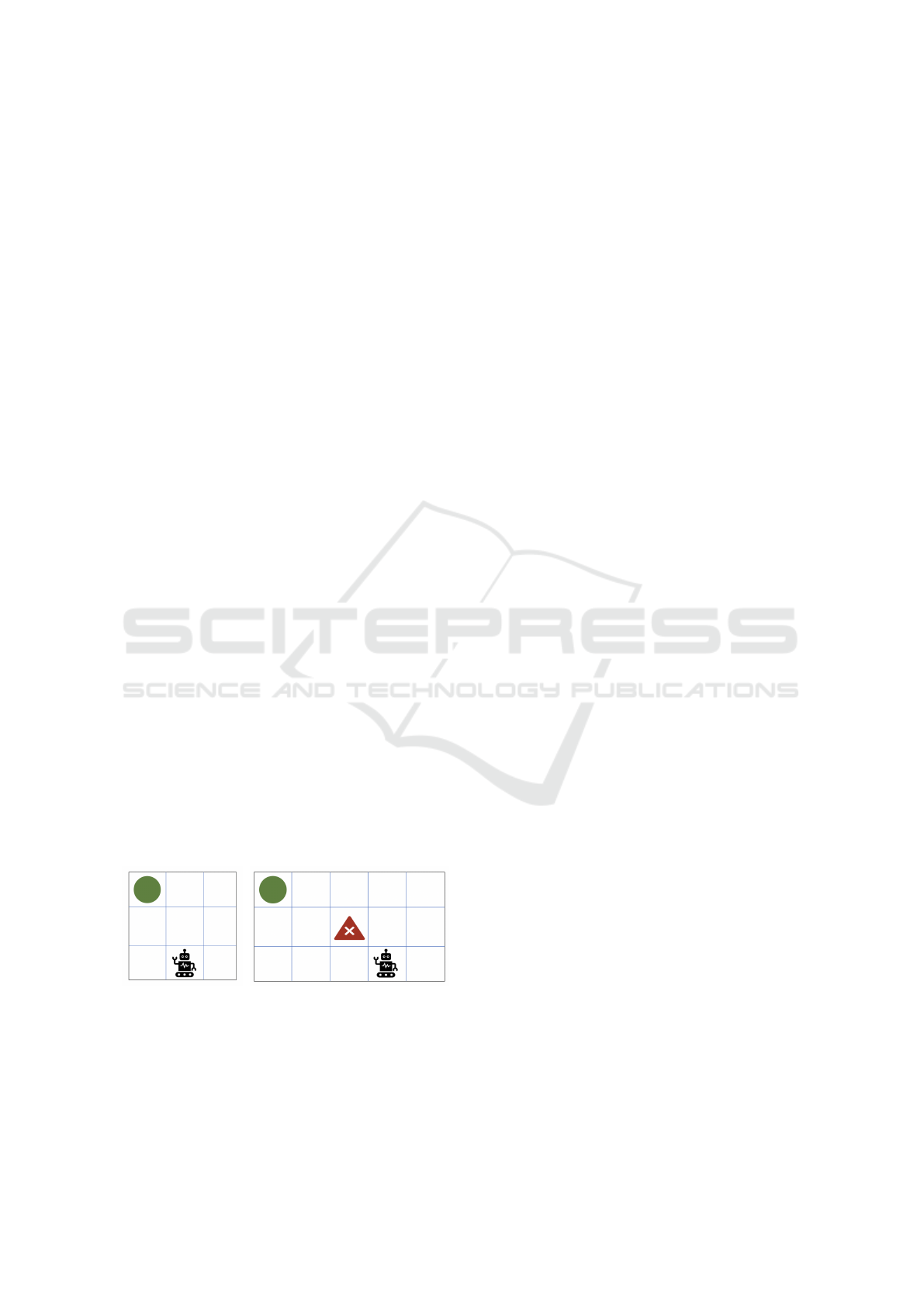
To evaluate our approach, we implemented a discrete
n × m multi-agent grid-world domain with i deter-
ministic rewards and i agents. At every time step t
each agent independently chooses an action from ac-
tion space A = {up, down, le f t, right, stand still}
depending on the policy π. More specifically, the
goal of every agent is to collect corresponding balls
while avoiding obstacles (e.g. walls and borders) and
penalty states (e.g. pits and others’ balls). The envi-
ronment size, number of agents, balls and obstacles
can be easily modified. Reaching a target location is
rewarded by a value of 220, whereas penalty states are
penalized by -220 and an extra penalty of -10 is given
for every needed step. An agent is done, when all
its corresponding balls were collected. Consequently,
we consider the domain as solved, when every agent
is done. The main goal lies in efficiently navigating
through the grid. Two example domains can be seen
in figure 2.
The starting position of all agents are chosen ran-
domly at the beginning of each episode whereas the
locations of their goals are fixed. The observation is
one-hot-encoded and divided into two layers. One
layer describes the agents’ position and its goal and
the other layer details the position of all other agents
and their goals. This observation is issued as input for
the algorithm. Therefore, the input shape is n×m×2.
To asses the learned policies, we use the accumulated
episode rewards as quality measure.
(a) 3x3 grid (b) 5x3 grid
Figure 2: Example figures of two single-agent domains.
Picture a) shows a 3 × 3 grid domain with one reward,
whereas b) illustrates a bigger 5 × 3 grid domain with an
additional penalty state.
4.2 Single-agent Results
First, we evaluate how adding an experience replay
buffer (ERB) and separating policy and target net-
work influences the learning process and performance
of a single agent. We started by running the tradi-
tional Q-RL algorithm as proposed by Neumann et
al. (2020) (Neumann et al., 2020) including their pa-
rameter setting. Then, we only added an experience
replay buffer (ERB) respectively solely the target net-
work. Finally, we extended the original algorithm
with a combination of both, an ERB and target net-
work. The resulting rewards on running all four ar-
chitecture on the 3 × 3 domain (see figure 2) can be
seen in figure 3 a) and the corresponding learned pol-
icy in figure 3 b). All graphs have been averaged
over ten runs. The traditional Q-RL agent without
any extensions (blue line) learns unstable with occa-
sional high swings down to -1700 and -1000 reward
points. Extended versions seem to be show less out-
liers. This observation gets more evident, when con-
ducting the same experiment on a bigger 5 × 3 en-
vironment. As seen in figure 3 c) - d) the achieved
rewards of non-extended agents (blue) collapses fre-
quently. The ERB (black) respectively target network
(green) alone stabilize learning, but the combination
of both (red) yields smoothest training curve. Hence,
these enhancements are getting more important with
bigger state space and more complex environments.
After training, we evaluate the resulting policies
for 100 episodes without further training. The av-
erage rewards of ten test-runs on the 3 × 3 domain
can be seen in figure 3 b). As already described, an
agent is rewarded +220 points for reaching its goal
and -10 for each taken step. So, when considering
an optimal policy, the agent would be awarded +190
for the 3 × 3 domain (respectively +170 for 5 × 3) if
the agent is spawned furthest from its goal and +220
for the best starting position. Assuming the starting
positions over all episodes are distributed evenly, the
optimal median reward would be at +205 for the 3×3
domain and +195 for the 5 × 3 environment.
The traditional QBM agent shows multiple out-
liers and a higher spread of rewards throughout the
evaluation episodes compared to the other architec-
tures. As it can be seen, adding only one of the ex-
tensions leads to a better median reward and a seem-
ingly optimal policy is gained through a combination
of both. Again, this observation gets more distinct
with bigger domains, see figure 3 d). Even though
ERB or target network alone significantly enhance
the median reward, the plots still show outliers. The
combined architecture is free of outliers with less in-
terquartile range and lower overall span indicating re-
ICAART 2022 - 14th International Conference on Agents and Artificial Intelligence
126
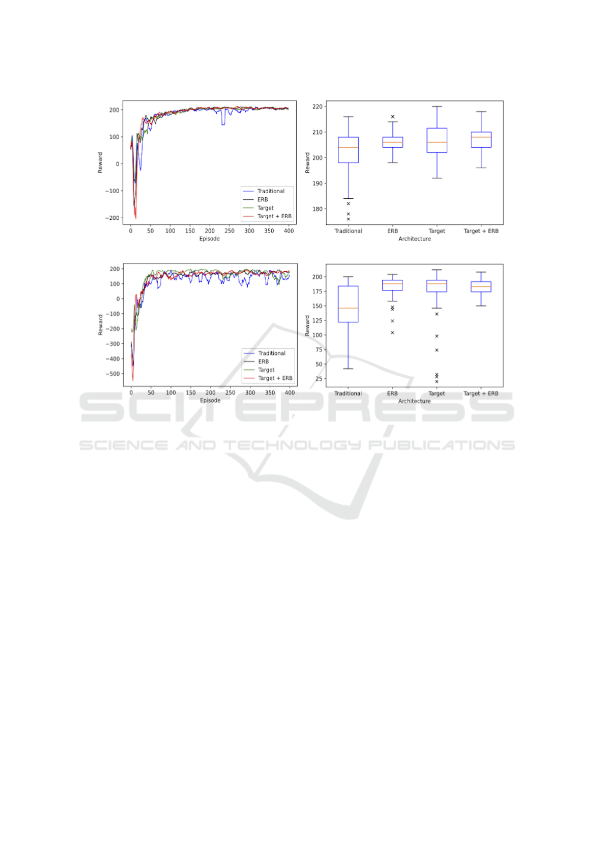
(a) Training: Reward per Episode (3x3) (b) Evaluation: Boxplot of Rewards (3x3)
(c) Training: Reward per Episode (5x3) (d) Evaluation: Boxplot of Rewards (5x3)
Figure 3: Performance of a single agent with different architectures. a) Shows the gained reward per episode on a 3 × 3
domain of different architectures, whereas b) displays the corresponding achieved rewards of the learned policy on 400 test
episodes. c) illustrates the reward of the same experiment on a 5 × 3 domain and d) the corresponding learned policy of test
episodes.
duced variance of training performance and nearly
optimal policy. In summary, alleviating data correla-
tion and the problems non-stationary distributions by
randomly sampling previous transitions and separat-
ing target and policy network increases stable learning
leading to robust and more optimal policies. Compar-
ing the results for 3 × 3 with the 3 × 5 gridworld, a
correlation of impact through the extensions and in-
put size can be suspected.
4.3 Multi-agent Results
Traditional Q-RL was limited so 2 ×2 multi-agent do-
mains and bigger domains could not be solved ratio-
nally (Neumann et al., 2020). This section explores,
if the proposed architecture enables multi-agent rein-
forcement learning. We modify the known environ-
ments by adding one agent and one corresponding
goal. If an agents picks up the others goal, it is pe-
nalized with -220. The averaged results over 10 runs
can be seen in figure 4.
The graphs suggest, that 3 × 3 domain (blue) can
be solved in contrast to the bigger environment (red).
Looking at figure 4 b), the median reward of the
learned policy on the smaller domain is around +350,
which is near optimum. Unfortunately, the bigger do-
main could not be solved with a median reward of
-450. Additionally, the 5 × 3 learning curve does not
seem to converge. Therefore, we can conclude, that
it is possible to solve bigger domains with the pro-
posed architecture, but Q-RL with ERB and extra tar-
get network still fails in somewhat larger multi-agent
domains.
Lastly, we explore if the cooperation method of
parameter sharing enhances quantum multi-agent re-
inforcement learning. With parameter sharing no
explicit communication is necessary since only one
centralized entity is trained and shared between the
agents. More specifically, the experience of every
agent is stored in a centralized ERB. At each train-
ing step, one QBM is trained with a randomized sam-
ple from the ERB similar to the single-agent case.
Towards Multi-agent Reinforcement Learning using Quantum Boltzmann Machines
127
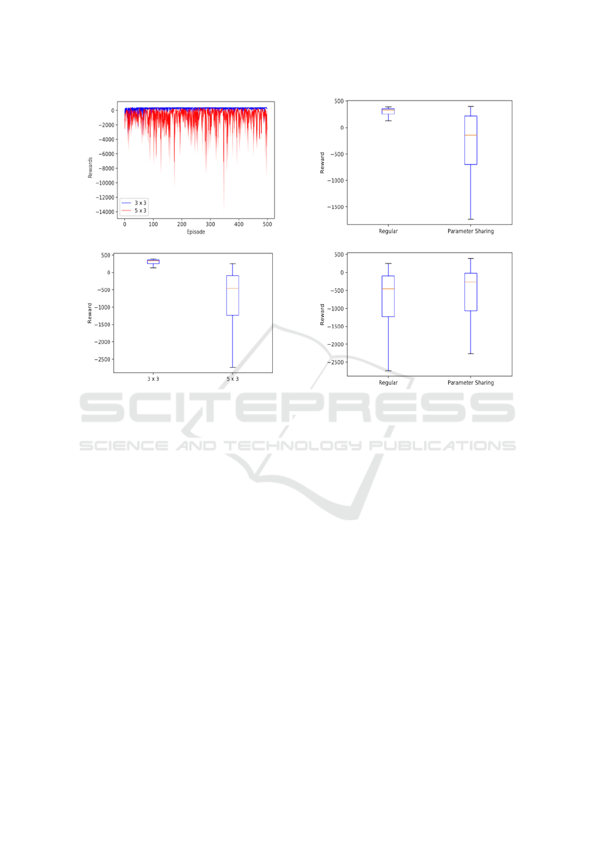
a) Learning Process on Both Domains
b) Learned Policy on Both Domains
Figure 4: Performance of two agents on the 3 × 3 (blue) re-
spectively 3 × 5 (red) domain. Figure a) shows the learning
process over 500 episodes, whereas figure b) displays the
learned policy over 100 testing episodes.
Both agents use this network to independently calcu-
late their Q-values based their observation. By this,
we additionally smooth the data distribution hoping
to achieve a more general policy and not two specific
policies adjusted to particular observations.
The results with and without parameter sharing
are illustrated in figure 5. Unfortunately, parameter
sharing seems to have a negative effect on the small
3 × 3 domain. In this case, the agents seem to have
learned a worse policy with this adaption. Rewards
on the bigger environments have increased. However,
the 5 × 3 domain can still not be considered solved.
Hence, parameter sharing is sub-optimal for the eval-
uated use case.
The complexity of the task and size of the in-
put did not increase, so this observation is counter-
intuitive. Since the centralized entity is simultane-
ously learning two independent behaviors, it might be
possible that in this case two independently optimal
action-state probability distributions (as learned with-
out parameter sharing) cancel out each other when
learned together. To proof this assumption, more ex-
periments must be conducted.
a) Learned Policy (3x3)
b) Learned Policy (5x3)
Figure 5: Performance of a two agents with and without pa-
rameter sharing. a) Shows the gained reward of the learned
policy of 100 testing episodes on a 3 × 3 domain, whereas
b) displays the same experiment on the bigger environment.
5 DISCUSSION
In summary, adding an ERB and additional target
network alleviates data correlation and the problem
of non-stationary distribution resulting in stabilized
learning and a more optimal policies. With the pro-
posed architecture, we were able to solve bigger
environments compared to traditional MARL using
QBMs. However, this architecture is still limited to
relatively small domains.
Even though it is possible to coordinate a single
agent in the 5 × 3 domain and multiple agents in a
smaller domain. The question remains why the 5 × 3
multi-agent domain fails. The QBM-agent receives
an input of 15 neurons on 5 × 3 single-agent domain
since only one input layer is needed. When adding
more agents to the environment, there is another in-
put layer necessary in order to distinguish between
the acting agent and other opposing agents. Hence,
the 3 × 3 multi-agent domain returns an observation
size of 18 and bigger multi-agent domain of size 30.
The input are considered in the QUBO formulation,
ICAART 2022 - 14th International Conference on Agents and Artificial Intelligence
128

which therefore increases. Hence, simulated quan-
tum annealing is applied to a bigger formulation. A
bigger formulation demands more qubits, which may
limit the accuracy, variation and stability of the quan-
tum annealing algorithm. This is only an assumption
and needs to be examined more closely. Neumann et
al. (2020) also already stated, that Q-RL is limited
by the current Quantum Processing Unit (QPU) size.
However, with the extension of an Experience Replay
Buffer and Target Network, we are able to stabilize
learning and therefore may reduce the needed QPU
size compare to previous approaches.
Quantum sampling has been proven to be a
promising method to enhance reinforcement learn-
ing tasks to speed-up learning in relation to needed
time steps (Neumann et al., 2020). Further work con-
cerning the relation between QPU size and domain
complexity (respectively state input) would needed to
strictly determine current limitations.
ACKNOWLEDGEMENTS
This work was funded by the BMWi project PlanQK
(01MK20005I).
REFERENCES
Ackley, D. H., Hinton, G. E., and Sejnowski, T. J. (1985). A
learning algorithm for boltzmann machines. Cognitive
Science, 9(1):147 – 169.
Benedetti, M., Realpe-G
´
omez, J., and Perdomo-Ortiz, A.
(2018). Quantum-assisted helmholtz machines: A
quantum–classical deep learning framework for in-
dustrial datasets in near-term devices. Quantum Sci-
ence and Technology, 3(3):034007.
Biamonte, J., Wittek, P., Pancotti, N., Rebentrost, P., Wiebe,
N., and Lloyd, S. (2017). Quantum machine learning.
Nature, 549(7671):195–202.
Binmore, K. (2007). Game Theory: A Very Short Introduc-
tion. Oxford University Press.
Charpentier, A., Elie, R., and Remlinger, C. (2020). Rein-
forcement learning in economics and finance.
Crawford, D., Levit, A., Ghadermarzy, N., Oberoi, J. S.,
and Ronagh, P. (2019). Reinforcement learning using
quantum boltzmann machines.
Foerster, J. N., Assael, Y. M., de Freitas, N., and Whiteson,
S. (2016). Learning to communicate with deep multi-
agent reinforcement learning.
Foerster, J. N., Farquhar, G., Afouras, T., Nardelli, N., and
Whiteson, S. (2017). Counterfactual multi-agent pol-
icy gradients. In AAAI.
Jerbi, S., Trenkwalder, L. M., Nautrup, H. P., Briegel, H. J.,
and Dunjko, V. (2020). Quantum enhancements for
deep reinforcement learning in large spaces.
Jumper, J., Evans, R., Pritzel, A., Green, T., Figurnov,
M., Tunyasuvunakool, K., Ronneberger, O., Bates,
R.,
ˇ
Z
´
ıdek, A., Bridgland, A., Meyer, C., Kohl, S.
A. A., Potapenko, A., Ballard, A. J., Cowie, A.,
Romera-Paredes, B., Nikolov, S., Jain, R., Adler,
J., Back, T., Petersen, S., Reiman, D., Steinegger,
M., Pacholska, M., Silver, D., Vinyals, O., Senior,
A. W., Kavukcuoglu, K., Kohli, P., and Hassabis, D.
(2020). High accuracy protein structure prediction us-
ing deep learning. In Fourteenth Critical Assessment
of Techniques for Protein Structure Prediction (Ab-
stract Book), 14.
Kiran, B. R., Sobh, I., Talpaert, V., Mannion, P., Sallab, A.
A. A., Yogamani, S., and P
´
erez, P. (2020). Deep rein-
forcement learning for autonomous driving: A survey.
Levit, A., Crawford, D., Ghadermarzy, N., Oberoi, J. S.,
Zahedinejad, E., and Ronagh, P. (2017). Free energy-
based reinforcement learning using a quantum proces-
sor.
Li, R. Y., Di Felice, R., Rohs, R., and Lidar, D. A. (2018).
Quantum annealing versus classical machine learning
applied to a simplified computational biology prob-
lem. npj Quantum Information, 4(1).
Mahmud, M., Kaiser, M. S., Hussain, A., and Vassanelli,
S. (2018). Applications of deep learning and rein-
forcement learning to biological data. IEEE Trans-
actions on Neural Networks and Learning Systems,
29(6):2063–2079.
Mcclelland, J., Mcnaughton, B., and O’Reilly, R. (1995).
Why there are complementary learning systems in the
hippocampus and neocortex: Insights from the suc-
cesses and failures of connectionist models of learning
and memory. Psychological review, 102:419–57.
Mirhoseini, A., Goldie, A., Yazgan, M., Jiang, J., Songhori,
E., Wang, S., Lee, Y.-J., Johnson, E., Pathak, O., Bae,
S., Nazi, A., Pak, J., Tong, A., Srinivasa, K., Hang, W.,
Tuncer, E., Babu, A., Le, Q. V., Laudon, J., Ho, R.,
Carpenter, R., and Dean, J. (2020). Chip placement
with deep reinforcement learning.
Mnih, V., Kavukcuoglu, K., Silver, D., Rusu, A., Veness, J.,
Bellemare, M., Graves, A., Riedmiller, M., Fidjeland,
A., Ostrovski, G., Petersen, S., Beattie, C., Sadik,
A., Antonoglou, I., King, H., Kumaran, D., Wierstra,
D., Legg, S., and Hassabis, D. (2015). Human-level
control through deep reinforcement learning. Nature,
518:529–33.
Morita, S. and Nishimori, H. (2008). Mathematical founda-
tion of quantum annealing. Journal of Mathematical
Physics, 49(12):125210.
Neukart, F., Compostella, G., Seidel, C., von Dollen, D.,
Yarkoni, S., and Parney, B. (2017a). Traffic flow opti-
mization using a quantum annealer.
Neukart, F., Dollen, D. V., Seidel, C., and Compostella, G.
(2017b). Quantum-enhanced reinforcement learning
for finite-episode games with discrete state spaces.
Neumann, N., Heer, P., Chiscop, I., and Phillipson, F.
(2020). Multi-agent reinforcement learning using sim-
ulated quantum annealing.
Neven, H., Denchev, V. S., Rose, G., and Macready, W. G.
(2008). Training a binary classifier with the quantum
adiabatic algorithm.
Towards Multi-agent Reinforcement Learning using Quantum Boltzmann Machines
129

O’Neill, J., Pleydell-Bouverie, B., Dupret, D., and
Csicsvari, J. (2010). Play it again: Reactivation of
waking experience and memory. Trends in neuro-
sciences, 33:220–9.
Paparo, G. D., Dunjko, V., Makmal, A., Martin-Delgado,
M. A., and Briegel, H. J. (2014). Quantum speedup
for active learning agents. Physical Review X, 4(3).
Peng, J. and Williams, R. J. (1994). Incremental multi-
step q-learning. In Cohen, W. W. and Hirsh, H., edi-
tors, Machine Learning Proceedings 1994, pages 226
– 232, San Francisco (CA). Morgan Kaufmann.
Puterman, M. L. (1994). Markov Decision Processes: Dis-
crete Stochastic Dynamic Programming. John Wiley
& Sons, Inc., New York, NY, USA, 1st edition.
Rebentrost, P., Mohseni, M., and Lloyd, S. (2014). Quan-
tum support vector machine for big data classification.
Physical Review Letters, 113(13).
Rummery, G. and Niranjan, M. (1994). On-line q-
learning using connectionist systems. Technical Re-
port CUED/F-INFENG/TR 166.
Sallans, B. and Hinton, G. E. (2004). Reinforcement learn-
ing with factored states and actions. J. Mach. Learn.
Res., 5:1063–1088.
Silver, D., Huang, A., Maddison, C., Guez, A., Sifre, L.,
Driessche, G., Schrittwieser, J., Antonoglou, I., Pan-
neershelvam, V., Lanctot, M., Dieleman, S., Grewe,
D., Nham, J., Kalchbrenner, N., Sutskever, I., Lill-
icrap, T., Leach, M., Kavukcuoglu, K., Graepel, T.,
and Hassabis, D. (2016). Mastering the game of go
with deep neural networks and tree search. Nature,
529:484–489.
Strehl, A. L., Li, L., Wiewiora, E., Langford, J., and
Littman, M. L. (2006). Pac model-free reinforcement
learning. In Proceedings of the 23rd International
Conference on Machine Learning, ICML ’06, pages
881–888, New York, NY, USA. ACM.
Sutton, R. S. and Barto, A. G. (2018). Reinforcement Learn-
ing: An Introduction. A Bradford Book, Cambridge,
MA, USA.
Tan, M. (1993). Multi-agent reinforcement learning: In-
dependent vs. cooperative agents. In In Proceedings
of the Tenth International Conference on Machine
Learning, pages 330–337. Morgan Kaufmann.
Wiebe, N., Braun, D., and Lloyd, S. (2012). Quantum algo-
rithm for data fitting. Physical Review Letters, 109.
ICAART 2022 - 14th International Conference on Agents and Artificial Intelligence
130
