Interactive Input and Visualization for Planning with Temporal

Uncertainty

M. H

ohn

1 a

, M. Wunderlich

2 b

, K. Ballweg

2 c

, J. Kohlhammer

1,2 d

and T. von Landesberger

3 e

Fraunhofer IGD, Germany

Technische Universit

at Darmstadt, Germany

Universit

at zu K

oln, Germany

landesberger@cs.uni-koeln.de

Keywords:

Data Visualization, Interaction, Temporal Uncertainty, Visual Design, User Study.

Abstract:

Data with temporal uncertainty is ubiquitous in everyone’s life. Popular examples are holiday planning or train

trips. There are several approaches to visualize temporal uncertainty, but common research usually does not

take uncertainty into account, neither as input nor output. We propose a new approach that provides both an

interactive drawing for data with temporal uncertainty and their respective visualizations. The user can draw

both variable and ﬁxed activities and also has the possibility to set probability distributions and enter indeﬁnite

activities. A quantitative user study shows the need and suitability of our new approach.

1 INTRODUCTION

Uncertainty is ubiquitous in everyone’s life. In many

of the domains that feature data and information with

uncertainty (e.g. physics, meteorology or the method

of data collection itself (Greis et al., 2017)), tempo-

ral information plays an important role (MacEachren

et al., 2012) (e.g., the start of a rain period). A typical

use case familiar to many people (soon again) is the

planning of a holiday trip.

A planned trip can be delayed already at the start,

i.e. a delayed outbound ﬂight or trafﬁc jams, and

after further potential issues during the trip, the end

becomes increasingly difﬁcult to predict. In general,

a temporal activity consists of three components that

can be categorized as ”Start” (S ), ”Duration” (D), and

”End” (E ). For a certain activity, these three com-

ponents are in the relation S + D = E to each other.

Therefore, each component is determined by the other

two parts. Usually, each of these three components

can be uncertain, complicating the relation between

S , D, and E signiﬁcantly.

Scheduling is the planning of times, at which par-

https://orcid.org/0000-0001-7732-0721

https://orcid.org/0000-0003-1510-733X

https://orcid.org/0000-0002-6835-9314

https://orcid.org/0000-0003-1706-8979

https://orcid.org/0000-0002-5279-1444

ticular activities will happen (Pinedo, 2012). It usu-

ally refers to future activities – in general as well as

in personal use. For each of the three components

(S , D and E ) of an activity we differentiate between

variable (e.g. ‘in between 12:30h and 13:30h’) and

ﬁxed (e.g. ‘either at 12:30h or at 13:30h’) occur-

rences. A variable activity could be a sightseeing trip

during the holiday, which lasts between four and ﬁve

days, whereas a ﬁxed activity could be the ﬂight it-

self, which starts either at 12:30h or at 13:30h. Fur-

thermore, a probability distribution can be set for the

uncertain components. If a probability distribution is

known, it can be either cumulative (e.g. ‘the activity is

expected to end at 13:15h, but may last until 13:30h’)

or discrete (e.g. ‘the activity ends at 12:30h with 70%

or at 13:30h with 30% probability’).

To draw activities with temporal uncertainty and

a probability distribution, users must be able to ex-

ternalize their internal knowledge. Often, users are

not able to quantify the temporal uncertainty (Lip-

kus et al., 2001; Wallsten et al., 1988; Shipman and

Marshall, 1999). An interactive visual method can

help to give this input in a faster and more reason-

able way (Greis et al., 2017). There are several, al-

ready evaluated approaches to visualize uncertainty

in general (MacEachren et al., 2012; Chittaro and

Combi, 2001; Hullman et al., 2019; Boukhelifa et al.,

2012) and visualizations for temporal uncertainty in

speciﬁc (Aigner et al., 2005; Gschwandtner et al.,

Höhn, M., Wunderlich, M., Ballweg, K., Kohlhammer, J. and von Landesberger, T.

Interactive Input and Visualization for Planning with Temporal Uncertainty.

DOI: 10.5220/0010761900003124

In Proceedings of the 17th International Joint Conference on Computer Vision, Imaging and Computer Graphics Theory and Applications (VISIGRAPP 2022) - Volume 3: IVAPP, pages 27-37

ISBN: 978-989-758-555-5; ISSN: 2184-4321

2016). Commercial solutions like Microsoft Project

provide options to quantify activities as optimistic or

pessimistic as well as PERT-like network diagrams

to visualize uncertainty within a schedule (Microsoft,

2021). Nevertheless, none of these approaches offer

a complete solution for drawing, editing and visualiz-

ing schedules containing activities with temporal un-

certainty to externalize implicit knowledge.

With our new approach, we provide the following

contributions:

• An extension of existing methods for visualizing

temporal uncertainty that enables the user to dis-

play

– certain and uncertain activities

– ﬁxed and variable components of activities

– indeﬁnite activities

– probability distributions for uncertain compo-

nents.

• A sketch-based interface to enter schedules that

include both certain and uncertain activities with

all the above characteristics.

• A quantitative user study to evaluate both the sys-

tem usability and the user performance. There-

fore, the study was spilt into two tasks: a drawing

assignment and a reading assignment.

2 RELATED WORK

The visualization of time-dependent data and sched-

ules is a well researched problem.

Charts and Diagrams. Gantt charts are one of the

most common visualization techniques used for plan-

ning activities (Aigner et al., 2011). Each activity

is represented by a bar. Its left-most position on a

time axis represents the start, whereas the width rep-

resents the duration of an activity. The description of

the activity can be displayed as textual labels in the

left part of the diagram or within their respective ac-

tivities. The main advantage of Gantt charts is their

simplicity and the similarity to bar charts, which are

intuitive and self-explanatory (Cleveland and McGill,

1986; Marty, 2009). Nevertheless, Gantt charts are

not suitable to visualize activities containing temporal

uncertainty, since every bar has a ﬁxed position, i.e. a

ﬁxed start and a ﬁxed duration (Aigner et al., 2005).

To overcome this drawback, several approaches have

been developed, that form a good foundation for our

new research.

Program Evaluation and Review Technique

(PERT) diagrams were developed in 1958 (Cook,

1966) and are used for scheduling tasks since then

(Merten, 1966; Bifﬂ et al., 2005). In a PERT diagram,

an activity is visualized as a table with the following

properties:

• earliest starting time (EST) and earliest ﬁnishing

time (EFT)

• latest starting time (LST) and latest ﬁnishing time

(LFT)

• a (minimal) duration and a buffer time

The buffer time describes the difference between

the minimal and the maximal duration of the activity.

With these properties, a PERT diagram is able to vi-

sualize certain activities (EST = LST and EFT = LFT

→ buffer time = 0) as well as activities with temporal

uncertainty (EST < LST and EFT < LFT → buffer

time > 0). A complete schedule consists of several

single PERT diagrams, where constraints can be visu-

alized as arrows, similar to Gantt charts. Although the

PERT diagrams can be arranged in a temporal order,

it is not trivial to determine the whole time span of

a schedule (Kosara and Miksch, 2002). Besides this

issue, the missing visualization is the obvious disad-

vantage, because all properties are represented as text

labels (Aigner et al., 2005).

In 2005, Aigner et al. presented a new technique

that combines the advantages of Gantt charts and

PERT diagrams – the PlanningLines (Aigner et al.,

2005). PlanningLines are designed as bars similar to

Gantt charts. Accordingly, the scalability for large

project plans has also been maintained. They also

allow the visualization of uncertainty with the same

properties as in PERT diagrams. The start interval be-

tween EST and LST is visualized as an open bracket

and the end interval between EFT and LFT as a clos-

ing bracket. The (minimal) duration of the activity is

visualized as a dark bar within these brackets. The

optional buffer time is visualized as a lighter-shaded

extension of the respective bar, divided equally be-

tween both ends.

Drawing. For an interactive input of uncertainty

Greis et al. (Greis et al., 2017) developed a set of

different sliders to quantify uncertainty. The sliders

provide different conﬁgurations to specify uncertain-

ties with several degrees of freedom. They also pro-

vide a good baseline for the latest research (Kleemann

and Ziegler, 2020) as well as our development. Since

most visualizations and periphery are based on a 2D

interface (Wang et al., 2013) a sketch-based input

is already used in scientiﬁc ﬁelds like mathematics

(LaViola Jr and Zeleznik, 2004; Zeleznik et al., 2008)

for more than 15 years. Furthermore, sketch-based

IVAPP 2022 - 13th International Conference on Information Visualization Theory and Applications

interfaces are especially suitable for application ar-

eas with predominantly beginners and inexperienced

users (Wang et al., 2013; Zheng et al., 2021). Lee et

al. presented a system to support users during sketch-

ing (Lee et al., 2011) with dynamic shadows, to give

them an idea of a possible outcome. This technique

is still used in modern research (Ghosh et al., 2019;

Shen et al., 2021).

Uncertainty Visualization. To visualize (temporal)

uncertainty several studies were conducted (Aigner

et al., 2005; Correll and Gleicher, 2014; Greis

et al., 2017; Lee et al., 2011; Wang et al., 2013).

MacEachren et al. evaluated eleven techniques (e.g.

location, orientation or fuzziness) and several icons to

visualize temporal and spatial uncertainty. As a main

result, they propose that icons are not suitable to vi-

sualize any kind of uncertainty, since pictorial repre-

sentations require an understanding of the underlying

uncertainty on the part of the viewer and the viewer

must also be able to correctly interpret the metaphor

of the icon (MacEachren et al., 2012). Instead, they

recommend the use of uncertainty visualisation tech-

niques that introduce a small error into the data but,

on the other hand, provide a faster assessment of the

uncertainty presented.

Gschwandtner et al. conducted a survey

to evaluate visualizations for temporal uncertainty

(Gschwandtner et al., 2016). The main aspect of

this survey was to assess which visualization should

be used for quantitative uncertainty (with knowl-

edge about the probability distribution) and qualita-

tive uncertainty (without such knowledge). The sur-

vey shows that for quantitative uncertainty, a gradi-

ent brush performs best but is not the favourite visu-

alization among the participants. For qualitative un-

certainty, ambiguation performs best and is also the

favourite visualization among the participants. Since

Aigner et al. uses ambiguation to visualize the buffer

time in their PlanningLines and the results are also

used in recent publications (Sondag et al., 2020; Pro-

copio et al., 2021), we decided to use these techniques

to visualize the uncertain parts of our visualization.

Finally, error bars are often used to visualize un-

certainty in data, but are often misinterpreted by users

(Correll and Gleicher, 2014; Hofman et al., 2020).

Furthermore, error bars are frequently associated with

high certainty in the data (Belia et al., 2005) and value

labels inside the bars are usually assumed to be more

certain than value labels outside (Newman and Scholl,

2012). To avoid this kind of incorrect interpretation

of the visualization, we use brackets instead of error

bars, similar to Aigner et al. (Aigner et al., 2005), to

visualize the time span of an activity.

Figure 1: A Tube with its attributes. The time span of the

activity is limited by the start and end interval. The max-

imum duration consists of the minimum duration and the

buffer time.

3 VISUALIZATION METHOD

The visualization of activities with temporal uncer-

tainty is not trivial. As mentioned above, uncertainty

is ubiquitous in everyone’s life (MacEachren et al.,

2012) and especially in the planning of future activi-

ties. For example, a simple holiday trip with ﬁve ac-

tivities features a variety of temporal uncertainties.

1. A ﬂight to the destination has a ﬁxed S and D,

and thus ﬁxed E

2. Packing a suitcase before the trip takes at least one

day.

3. Sightseeing during the holidays for at least four

days but maximum ﬁve days

4. A two-day trip during the holidays

5. The return ﬂight is expected to take place on the

scheduled day, but could be delayed by one day

due to a pilot strike

Such schedules and taxonomies (Shneiderman,

2003; Gschwandtner et al., 2012) suggest the follow-

ing visualization characteristics to be fulﬁlled by the

design of our new approach:

C1 certain activities

C2 uncertain activities with a certain S and uncer-

tain E interval and vice versa

C3 uncertain activities with an open S or open E

(indeﬁnite activities)

C4 both certain and uncertain activities within a

time span

C5 ﬁxed characteristics for S , D and E

C6.1 a cumulative probability distribution for S , D

and E

C6.2 a discrete probability distribution for S , D and

C7 dependencies between two activities

PlanningLines (Aigner et al., 2005) already pro-

vides a good basis to visualize activities with tem-

poral uncertainty, especially C1, C2 and C4 are al-

Interactive Input and Visualization for Planning with Temporal Uncertainty

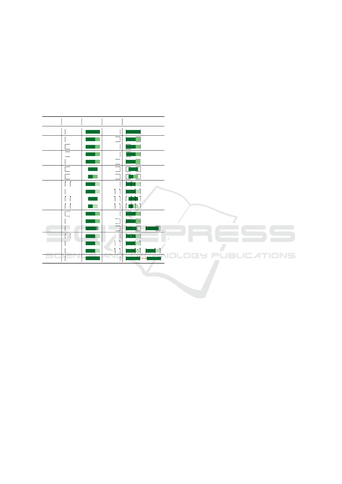
Table 1: Representative conﬁgurations of Tubes according

to the characteristics (Char.) C1–C7. For C5

†

, the buffer

time has to be used, if the ﬁrst possible start is taken. The

rows marked with ∗ each show two representatives with

different probability distributions. C6.1

∗

shows activities,

which are probable ﬁnished after 25% or 75% of the buffer

time. C6.2

∗

shows activities for which the whole buffer time

happens with a probability of 25% or 75%. In C7, the de-

pendency between two activities is visualized by an orange

arrow.

Char. S D E Representative

†

C6.1

∗

C6.2

∗

ready supported. Although Aigner et al. provide sim-

ple projects plans with uncertainty in their publica-

tion, their approach does not support interactive input

and differs in various visual aspects as detailed be-

low. Thus, we slightly modify their components to

present the opportunity for an interactive drawing as

well as the editing of activities within a schedule. We

named our new development Tube. A schematic rep-

resentation of a tube with all its attributes is shown in

Fig. 1. Examples for different conﬁgurations of Tubes

fulﬁlling the Characteristics C1–C7 are shown in Ta-

ble 1. As PlanningLines were already successfully

evaluated (Aigner et al., 2005), the formal constraints

and properties of them were adopted. The temporal

attributes were also adopted to visualize the S, D and

E properties of an uncertain activity (see Fig. 1). The

start interval is limited by the earliest starting time

[EST] and the latest starting time [LST], the end inter-

val is limited by the earliest ﬁnishing time [EFT] and

the latest ﬁnishing time [LFT] and the maximum du-

ration of an activity is deﬁned by the minimum dura-

tion and the buffer time – the time difference between

the maximum and the minimum duration.

The major visual difference between Planning-

Lines (Aigner et al., 2005) and Tubes is the visual-

ization of the buffer time. Usually, PlanningLines

divides the buffer time equally between both ends.

In contrast, we designed our Tubes with the buffer

time always visualized on the right side of the min-

imum duration to foster easier understanding. The

user therefore does not have to add two parts of the

buffer time, but can perceive it at once.

As written above, PlanningLines already covers

some requirements of the characteristics. To sup-

port the remaining demands, several combinations

of the visual variables for visualizing uncertainty by

MacEachren (MacEachren et al., 2012) are used. To

ﬁnd a good solution, we created several sketches in

an iterative process on a whiteboard (Roberts et al.,

2015) and discussed them during the development of

our system.

Indeﬁnite activities (C3) are visualized with an

open bracket on the open side. Therefore, the hori-

zontal lines are the remaining parts to foster a more

intuitive understanding. To support C5, D is visual-

ized with a texture for a discrete setting. S and E

are visualized as arrows with the direction of the ar-

rowhead indicating whether it is about S or E . For a

variable activity with a known probability distribution

of S , D or E , a cumulative distribution function is

chosen to visualize the user input using a linear gradi-

ent brush (C6.1

∗

) (Fig. 5). The calculation is adapted

from Correl et al. (Correll and Gleicher, 2014). The

probability for a ﬁxed buffer time is represented by

a chessboard texture. The granularity is varied based

on the set probability, so less probable buffer time is

sparser than more probable buffer time (C6.2

∗

). For

cases when S has a known probability, ambiguation

is used, so a less probable ﬁxed start is visualized

in lighter colors than a more probable one. Differ-

ent conﬁgurations are shown in Fig. 6. This is also

applied to a discrete E .

4 APPLICATION

To support drawing, editing and visualizing activities

with temporal uncertainty, a system architecture was

developed. All user controls are grouped into three

categories within a menu bar. The main category pro-

vides the options for input and editing of Tubes (see

Section 4.1 & 4.2). The other categories contains I/O

features and several possibilities to personalize the

schedules. As an extension to Aigner et al. (Aigner

et al., 2005), we provide the means to draw and visu-

alize both continuous and discrete activities. Further-

IVAPP 2022 - 13th International Conference on Information Visualization Theory and Applications

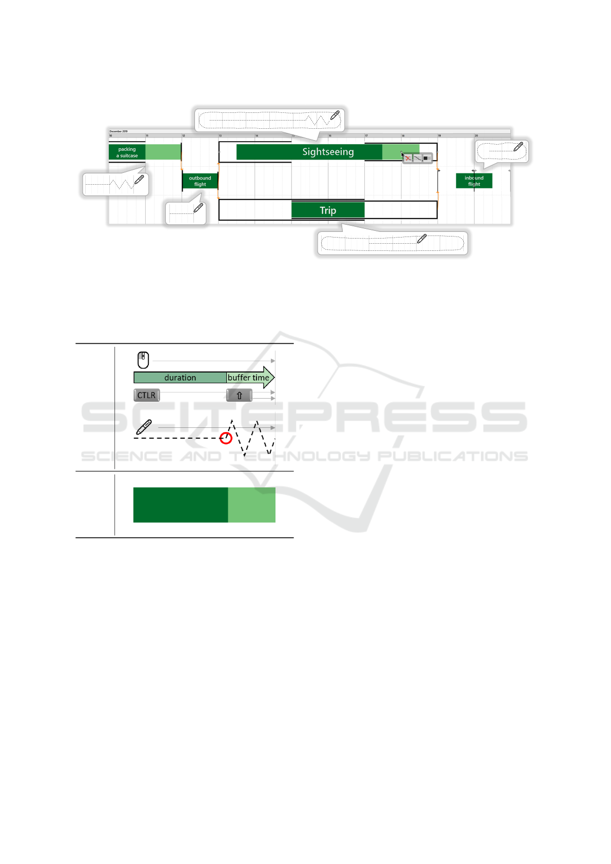
Figure 2: The ﬁgure shows a schedule of a holiday trip planned with temporal uncertainty. Our new Tubes visualize the

activities with different properties. The user can draw each activity with simple inputs. The corresponding drawing actions are

shown in the bubbles near each Tube. Furthermore, the mouse-sensitive context menu for editing is shown at the ”Sightseeing“

Tube.

Table 2: Drawing an uncertain activity with the different

input methods and the resulting Tube.

mouse

stylus

result

more, we also allow the input of probability distribu-

tion for all uncertain components of a Tube and offer

the possibility to draw indeﬁnite activities.

4.1 Input of Tubes

There are two possible methods to draw a single ac-

tivity: input with mouse and keyboard and input with

stylus on a tablet. For both methods, the user can en-

ter either a start interval, an end interval, or a duration

with an optional buffer time. If the time span of an ac-

tivity is known, the user can also enter a time range in-

stead of a start and end interval. The components are

drawn as shadows and after ﬁnishing the input of all

components the user receives suggestions for possible

Tubes (Fig. 3). A schematic representation for the in-

put of an uncertain duration with both input methods

is given in Table 2.

Drawing with Mouse and Keyboard. To draw an

activity with mouse and keyboard, the user has to use

the control (CTRL) and shift (⇑) buttons as modiﬁers.

The position of the mouse deﬁnes the position of an

activity within a schedule. The user can draw the du-

ration with the mouse while pressing the left mouse

button and move the mouse on a straight line. The

user can also draw Start, End and Range elements in

the same way. To draw a buffer time, the user starts

to enter a duration and presses the shift button addi-

tionally from the point where the buffer time should

start and moves the mouse with pressed left button as

far as the buffer time should go. During the sketching

process, all elements are classiﬁed due to their relative

position to each other, whereas the ﬁrst drawn element

is always classiﬁed as a duration element – regardless

of a possible buffer time. The user can monitor its

input due to the shadow drawing method (Lee et al.,

2011).

Drawing with a Stylus. Beside the input with

mouse and keyboard, a drawing method with a sty-

lus is also implemented to provide a compatibility

with modern touchscreen devices, e.g. tablets. In this

mode, the user can draw lines with the stylus, which

are automatically classiﬁed afterwards depending on

their shape. To enter a certain activity, the user has

to draw a straight line, similar to the movement of the

mouse in the alternative mode. Due to the circum-

stances that no keyboard or other additional devices

can be used to press certain keys as modiﬁers, the line

classiﬁer has to distinguish between certain and un-

Interactive Input and Visualization for Planning with Temporal Uncertainty

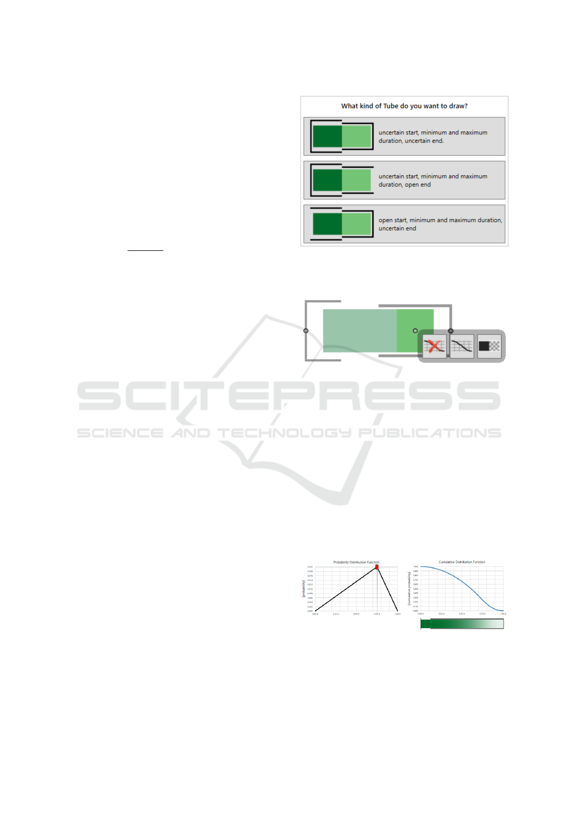
certain activities in a different way. If there is a point

with a slope |m| ≥ 1, then the buffer time applies from

this point onward (Table 2, red circle). Further input

elements, Start, End and Range, can be drawn and

are analysed by the classiﬁer. The following code out-

lines the classiﬁcation, where PC is an ordered collec-

tion of 2D points representing the internal structure of

the input. The algorithm ﬁrst extracts three important

points of PC: the ﬁrst point f , the last point l, and the

point d with the greatest horizontal distance from f .

1: f ← PC. f irst, l ← PC.last

2: d ← p ∈ PC with max(| f .x − p.x|)

3: if l = d then  D entered

4: m

←

.y−p

i+1

.x−p

i+1

, i ∈ {1, . . . , |PC| − 1}

5: if max(m

) > 1 then

6: return uncertain D

7: else

8: return certain D

9: end if

10: else  S, E or Range entered

11: if ∆( f , l) < τ then

12: return Range

13: else if d.x < f .x then

14: return Start

15: else if d.x > f .x then

16: return End

17: end if

18: end if

After classifying the input, the components are

displayed as shadows to support the user for further

input (Lee et al., 2011).

Transforming input into Tubes. After the draw-

ings are taken – either with mouse and keyboard or

with a stylus – and the input is formally correct, the

user gets suggestions for possibles Tubes depending

on the taken input. Since the input is only clearly de-

ﬁned through the triple of S , D and E , the user can

select the desired result Tube from a pop-up menu that

shows all possible combinations for the drawn com-

ponents. Fig. 3 shows an example of the user dialogue

for the possible Tubes with a drawn user input of a du-

ration (with buffer time) and a range.

4.2 Editing of Tubes

The editing of drawn Tubes is an important feature of

the interactive input of activities. Beside the trivial

actions like deleting or moving a Tube, more complex

operations for editing Tubes and creating dependen-

cies between two Tubes are implemented. In the cor-

responding editing mode of the software, the Tubes

have mouse-sensitive editing points on certain ele-

Figure 3: An example dialog for the supervised input. The

user has to choose the Tube he wants to draw with the input

of a duration and a range.

Figure 4: A context menu for editing of this Tube to change

the buffer time from a continuous to a discrete one (right),

add a new probability distribution (center), or remove a

probability distribution (left).

ments to open a context menu for editing a compo-

nent of a Tube. Fig. 4 shows this behaviour for the

buffer time of an activity. You can either change this

buffer time from variable to ﬁxed or the other way

round (right), add a probability distribution (center),

or remove a probability distribution (left).

Probability Settings. In some cases the user wants

to quantify the probability distribution of S , E or the

buffer time. After selecting the corresponding menu

item (see Fig. 4, center) a new user dialogue pops up

Figure 5: The user can set a known probability, whether

an activity is more likely to last longer or shorter, with a

slider in the probability distribution function (top left) and

sees the resulting cumulative probability function directly

(top right). Bottom shows the resulting Tube with the set

probability distribution in the buffer time visualized with a

gradient.

IVAPP 2022 - 13th International Conference on Information Visualization Theory and Applications

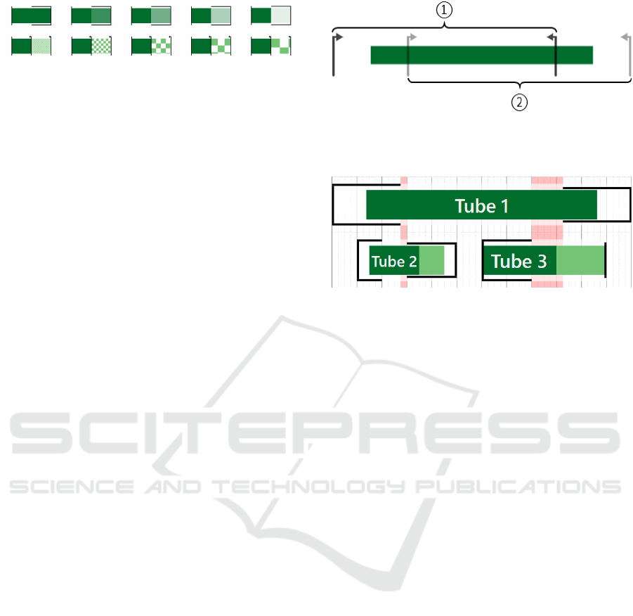
Figure 6: Tubes with a constant probability distribution

from 1.0 to 0.0 (top row, left to right) and Tubes with a

discrete buffer time and a respective probability from 1.0 to

0.0 (bottom row. left to right).

(Fig. 5) in which the user can set, whether the activity

is more likely to last longer or shorter. The expected

duration can be set with a slider in a probability dis-

tribution function (left, black). A cumulative distribu-

tion function (right, blue) shows the result of the input

directly. The cumulative distribution is converted into

a gradient (Correll and Gleicher, 2014) to show the

probability distribution in the resulting Tube (bottom).

The same technique can be use to quantify a probabil-

ity distribution for the start and end components of a

Tube (see Table 1).

Variable and Fixed Components. To quantify a

constant probability for the buffer time (‘every point

in time has the same probability’) or a probability for

ﬁxed components in an activity (S , D, or E ), the di-

alogue only has to offer one slider to set the desired

probability. The result for a constant probability with

a ﬁxed buffer time and different probabilities is shown

in Fig. 6. To visualize a quantitative probability for a

ﬁxed buffer time, we chose the technique grain by

MacEachren (MacEachren et al., 2012), where the

rule is: the less likely the buffer time, the sparser the

grid. For Tubes with a variable buffer time, the prob-

ability is mapped to the alpha value of the base color.

The target function has a value range from 0.1 to 1.0

to avoid totally transparent components (zero proba-

bility). The same color is chosen for the base color

and the color for the minimum time, so a buffer time

with 100% probability is visualized like the minimum

duration. Representatives for different probabilities

are shown in Fig. 6. For ﬁxed S and E components,

the same technique as for variable buffer time with a

constant probability is used. The components differ

in their alpha value, depending on the chosen proba-

bility (see Fig. 7).

4.3 Additional features

To avoid conﬂicts within a schedule, the application

has a built-in cross-check to highlight such risks. The

system examines the drawn Tubes pairwise after each

input to detect overlaps within the schedule. For this,

only the part of an activity that will certainly happen

is taken into consideration. If a conﬂict is detected,

Figure 7: Tube with discrete start and end and constant

probability. The activity happens with 70% in time span

(1) and 30% in time span (2).

Figure 8: In the red-marked time spans, the Tubes conﬂict

with each other, because Tube 1 and Tube 2, respectively

Tube 1 and Tube 3 deﬁnitely happen there in this schedule.

the corresponding time span will be highlighted with

a red marker (see Fig. 8). Furthermore, Tubes can

be moved on the x-axis to re-deﬁne their time span

within the schedule. They also can be moved on the

y-axis into a different layer to avoid overplotting. As

with PlanningLines (Aigner et al., 2005), the user also

has the opportunity to draw dependencies between

two activities (see Table 1, C7) to visualize that one

activity has to be ﬁnished before the other one can

start.

5 EVALUATION

We conducted a quantitative user study to evaluate

both the drawing input with our new application and

the corresponding visualization. Therefore, we di-

vided the study into two parts – a drawing assignment

to assess the potential of the input methods and the

application, and a reading assignment to evaluate the

visualization.

5.1 Experimental Setting

A total of 21 participants (10 male, 10 female, 1 pre-

ferred not to say) took part in the study. The age

distribution was between 20 and 71, but the major-

ity of the participants were between 20 and 30 years

old (67%). The participants came from different pro-

fessional ﬁelds, thus covering a broad spectrum of

users. The study took place as a laboratory study

and the conductor was present at all times to answer

Interactive Input and Visualization for Planning with Temporal Uncertainty

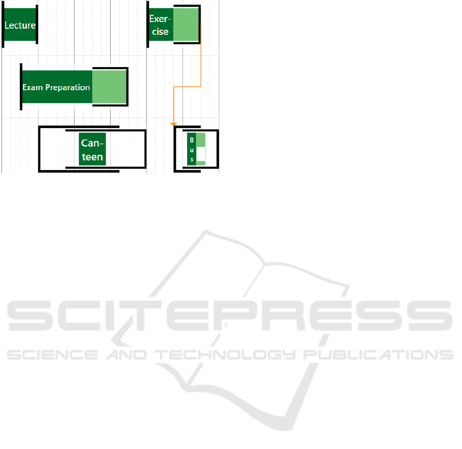
Figure 9: Tubes with different characteristics representing a

hypothetical day at a university.

upcoming technical questions. All participants used

the same technical equipment to ensure equal condi-

tions. The study was designed within-subject to gen-

erate a signiﬁcantly larger result set than in a between-

subject design with the same number of participants

(Charness et al., 2012). Thus, each participant worked

on all assignments. After a brief introduction to the

subject of the study and an explanation of the user in-

terface by the conductor, the participants started with

the study. There was no speciﬁc training phase, al-

though all participants were asked to use the built-in

help system to answer their questions concerning the

application and the visualization by themselves. Each

interview took between 60 and 150 minutes.

The initial setup of the study was to split the par-

ticipants into two groups – one group working on the

reading assignment ﬁrst and ﬁnishing with the draw-

ing assignment, and a second group working on the

study in reverse order. The hypothesis was that par-

ticipants would make fewer mistakes when drawing

if they had seen and understood the visualization be-

forehand. However, the initial evaluation of the study

showed that the groups had almost identical correct-

ness, suggesting that there is no signiﬁcant learning

effect. This led us to consider all participants as one

group for the result evaluation.

5.2 Assignments & Data

The drawing assignment addresses the newly devel-

oped software and its intuitiveness and robustness.

Beside the known use case (Fig. 2), a second sched-

ule had to be visualized (Fig. 9). For this schedule, a

hypothetical day at a university was created with the

following activities:

• Visit a lecture between 10:00am and 11:00am

• Exam preparation with fellow students at 10:30am

with an uncertain end between 12:30pm and

01:30pm

• Visit an exercise starting at 02:00pm with a dura-

tion of at least 45min. After 45min, the assign-

ments are probably not yet completed. However,

the chances increase with each minute. In any

case, the exercise will take a maximum of 90min.

• Go to the canteen for a maximum of 45min after

the lecture, but before the exercise starts

• Take the bus after the exercise. It will take either

15min or 30min, depending on the route.

For this assignment the participants were asked to

draw the two different schedules that were given to

them in a textual representation. Each schedule con-

sisted of ﬁve activities focusing on different speciﬁcs,

e.g. certain start and uncertain end, or activities con-

taining a probability distribution or discrete compo-

nents.

The participants were also given a reading assign-

ment as a prepared schedule with different activities,

drawn in advance by the conductor with the new ap-

plication. The shown schedule is a slightly modiﬁed

version of the project plan evaluated by Aigner et al.

in 2005 (Aigner et al., 2005) to ensure the compara-

bility of the evaluation results. We have varied the

activities so that all characteristics are represented by

at least one Tube. The schedule is depicted in Fig. 10.

This assignment was conducted to evaluate the

comprehensibility of the visualization. The partici-

pants were asked to answer questions on the details

of the visualizations, e.g. “When is the earliest pos-

sible start?”, “When is the latest possible end?” or

“What is the maximum duration of the activity?”.

Finally, the participants were asked to ﬁll in a form

for the system usability score by Sauro (Sauro, 2011).

5.3 Analysis

The drawing assignments were evaluated by the spe-

ciﬁc features of the Tubes to be drawn – an exist-

ing property was assigned a value of 1 and a miss-

ing property was assigned a value of 0. The read-

ing assignment was evaluated with 1 for a correct an-

swer and 0 for a wrong answer. Therefore, an average

correctness value of 1.0 means, that all participants

have fully met all requirements, while a value of 0.0

means, that no requirement was fulﬁlled by any par-

ticipant. The results are shown in Fig. 11 and are fur-

ther explained in the remainder of this section.

IVAPP 2022 - 13th International Conference on Information Visualization Theory and Applications

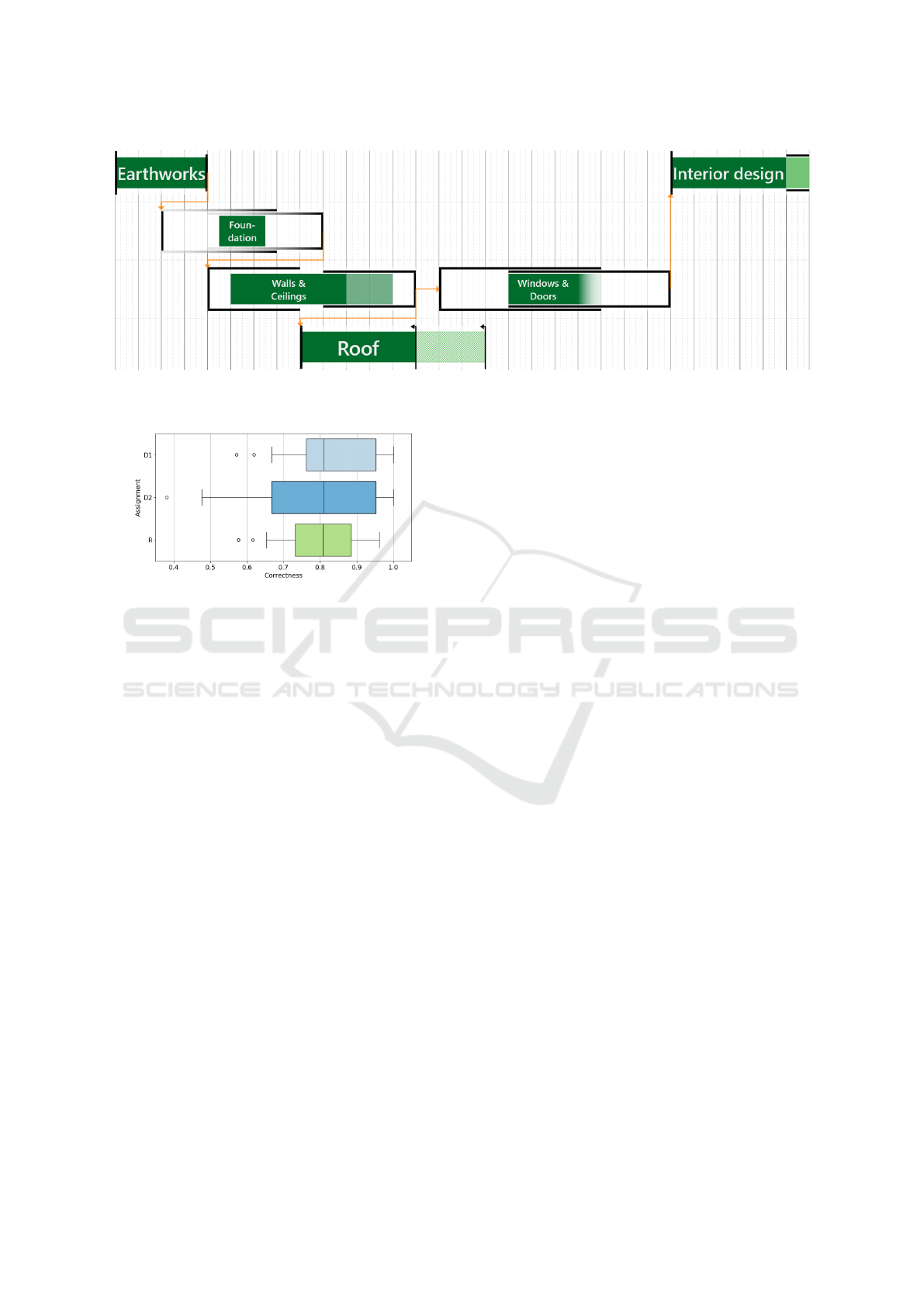
Figure 10: The example schedule of the reading assignment. The plan has been adopted from Aigner et al. (Aigner et al.,

2005) and slightly modiﬁed so that all characteristics can be queried.

Figure 11: Results of the drawing assignments (D1, D2) and

the reading assignment (R). The assignments had a similar

average rating, but differ strongly in the variance of the re-

sults.

Drawing Assignment. The two schedules (D1 - a

day at a university, D2 - the holiday use case) were

evaluated individually, followed by a comparison be-

tween them.

D1 has an average correctness of 0.8413. The only

activity with a comparably low correctness (0.7048)

was the bus transfer. The main problem was to set

the right start interval. The intended solution was an

uncertain start within 45min and 90min of the dura-

tion of the exercise ahead. Instead, eleven participants

drew a certain start right after the latest possible end-

ing of the exercise. Furthermore, the probability dis-

tribution for this ﬁxed and uncertain activity was not

set correctly in 12 of 21 cases. Another difﬁculty in

this schedule was to set the probability distribution for

the duration of the exercise in the right way – 10 of 21

participants had problems with that aspect.

D2 has an average correctness of 0.7755. The

main problems with this schedule came from the in-

deﬁnite activity of packing the suitcase (0.7738) and

the inbound ﬂight (0.6667). In the suitcase activity,

setting the right start was the main challenge, whereas

the inbound ﬂight causes multiple problems concern-

ing the maximal duration, the ﬁxed start and end in-

terval, and the probability distribution.

Both drawing assignments have exactly the same

median correctness value of 0.8095. This high num-

ber shows the good usability of the developed soft-

ware, in particular for new users. Participants did not

have much trouble entering certain activities, nor did

they have much difﬁculty entering uncertain activi-

ties within a time span. Problems occurred only with

activities with more speciﬁc properties, such as ﬁxed

components or probability distributions.

Reading Assignment. The reading assignments

has an average correctness of 0.7875. The results

show that users read the certain activity almost with-

out errors, just like the Tube with ﬁxed components.

Problems occurred with the indeﬁnite activity and its

open end. The main problems appeared around the

probability distributions and with the components S

and E , causing signiﬁcantly more problems for the

participants than such a characteristic in D.

Summary. The two different assignments show

similar performances for the different characteristics

of the Tubes. On the one hand, the participants had

problems with the probability distributions, both dur-

ing drawing and reading. This could be due to the

fact that judgements under uncertainty are often me-

diated by intuitive heuristics (Tversky and Kahneman,

1983). Furthermore, 10 participants drew constraints

between two activities. While this was not a task in

the assignments, it is a good point to consider in fu-

ture iterations of the research. On the other hand,

Tubes with other characteristics than probability dis-

tributions seemed to be no problem for the partici-

pants, both during drawing and reading. This obser-

vation is also reﬂected in the similar statistics for the

assignments (see Fig. 11). With an average correct-

ness of 0.8117, the study shows good results in both

drawing schedules with our software and visualiza-

tion.

Interactive Input and Visualization for Planning with Temporal Uncertainty

System Usability Score. The system usability

score indicates the subjective evaluation of the useful-

ness and utility of the application by the participants

(Sauro, 2011). The score of this evaluation for our

system is between 30.0 and 92.5. The average score

of 66.19 shows that our new application can be clas-

siﬁed as ‘OK’.

6 CONCLUSION AND FUTURE

WORK

We presented both a new visualization and a corre-

sponding application for the interactive visual input

for planning with temporal uncertainty. The visual-

ization is based on the PlanningLines approach by

Aigner et al. (Aigner et al., 2005). With our extension

of this approach, it is also possible to visualize both

variable and ﬁxed activities. Furthermore, it is possi-

ble to visualize different probability distributions and

indeﬁnite activities. For the interactive drawing of

schedules, the new application offers input methods

using both mouse and keyboard as well as stylus in-

put. After sketching a Tube, the user is supported with

shadow-drawing (Lee et al., 2011) to get suggestions

for the ﬁnal visualized Tubes. We conducted a quan-

titative user study to show the added value of the new

visualization and application. The drawing assign-

ments emphasize the beneﬁts of the new application

in externalising the temporal uncertainties. With the

reading assignment the suitability of the visualization

was shown. Furthermore, the user study showed that

the holiday use case example (see section 1) can be

externalized by the majority of the participants with-

out signiﬁcant issues. The objective evaluation shows

an average correctness of about 80% for both parts of

the study. Since no participant used the application

before the study took place, it can be assumed that

the accuracy will increase with regular use. To eval-

uate the subjective perception, the participants were

asked to ﬁll in a system usability score (Sauro, 2011).

The score shows, that the system can be classiﬁed as

‘OK’. Nevertheless, the broad range of scores shows

that we have to work on an even more user-friendly

way to enter complex conﬁgurations.

As upcoming steps, more functionality for edit-

ing tubes will be realized. This includes possibilities

to vary the durations of Tube components as well as

an advanced input dialogue to enter the probability

distributions in an easier way. Furthermore, we plan

extended quality-of-live improvements, like zooming

and panning, or individual colors for single Tubes to

provide more customizability for the schedule.

REFERENCES

Aigner, W., Miksch, S., Schumann, H., and Tominski, C.

(2011). Visualization of time-oriented data. Springer

Science & Business Media.

Aigner, W., Miksch, S., Thurnher, B., and Bifﬂ, S. (2005).

Planninglines: novel glyphs for representing tempo-

ral uncertainties and their evaluation. In Ninth In-

ternational Conference on Information Visualisation

(IV’05), pages 457–463.

Belia, S., Fidler, F., Williams, J., and Cumming, G.

(2005). Researchers misunderstand conﬁdence inter-

vals and standard error bars. Psychological methods,

10(4):389.

Bifﬂ, S., Thurnher, B., Goluch, G., Winkler, D., Aigner,

W., and Miksch, S. (2005). An empirical investiga-

tion on the visualization of temporal uncertainties in

software engineering project planning. In 2005 Inter-

national Symposium on Empirical Software Engineer-

ing, 2005., pages 10–pp. IEEE.

Boukhelifa, N., Bezerianos, A., Isenberg, T., and Fekete,

J.-D. (2012). Evaluating sketchiness as a visual vari-

able for the depiction of qualitative uncertainty. IEEE

Transactions on Visualization and Computer Graph-

ics, 18(12):2769–2778.

Charness, G., Gneezy, U., and Kuhn, M. A. (2012). Exper-

imental methods: Between-subject and within-subject

design. Journal of Economic Behavior & Organiza-

tion, 81(1):1–8.

Chittaro, L. and Combi, C. (2001). Representation of

temporal intervals and relations: information visual-

ization aspects and their evaluation. In Proceedings

Eighth International Symposium on Temporal Repre-

sentation and Reasoning. TIME 2001, pages 13–20.

Cleveland, W. S. and McGill, R. (1986). An experiment in

graphical perception. International Journal of Man-

Machine Studies, 25(5):491–500.

Cook, D. L. (1966). Program evaluation and review tech-

nique: Applications in education. Number 17. US De-

partment of health, education, and welfare, Ofﬁce of

education.

Correll, M. and Gleicher, M. (2014). Error bars considered

harmful: Exploring alternate encodings for mean and

error. IEEE transactions on visualization and com-

puter graphics, 20(12):2142–2151.

Ghosh, A., Zhang, R., Dokania, P. K., Wang, O., Efros,

A. A., Torr, P. H., and Shechtman, E. (2019). Inter-

active sketch & ﬁll: Multiclass sketch-to-image trans-

lation. In Proceedings of the IEEE/CVF International

Conference on Computer Vision, pages 1171–1180.

Greis, M., Schuff, H., Kleiner, M., Henze, N., and Schmidt,

A. (2017). Input controls for entering uncertain data:

Probability distribution sliders. Proc. ACM Hum.-

Comput. Interact., 1(EICS):3:1–3:17.

Gschwandtner, T., B

ogl, M., Federico, P., and Miksch, S.

(2016). Visual encodings of temporal uncertainty: A

comparative user study. IEEE Transactions on Visual-

ization and Computer Graphics, 22(1):539–548.

Gschwandtner, T., G

artner, J., Aigner, W., and Miksch, S.

(2012). A taxonomy of dirty time-oriented data. In

IVAPP 2022 - 13th International Conference on Information Visualization Theory and Applications

Quirchmayr, G., Basl, J., You, I., Xu, L., and Weippl,

E., editors, Multidisciplinary Research and Practice

for Information Systems, pages 58–72, Berlin, Heidel-

berg. Springer Berlin Heidelberg.

Hofman, J. M., Goldstein, D. G., and Hullman, J. (2020).

How visualizing inferential uncertainty can mislead

readers about treatment effects in scientiﬁc results. In

Proceedings of the 2020 CHI Conference on Human

Factors in Computing Systems, pages 1–12.

Hullman, J., Qiao, X., Correll, M., Kale, A., and Kay, M.

(2019). In pursuit of error: A survey of uncertainty

visualization evaluation. IEEE transactions on visual-

ization and computer graphics, 25(1):903–913.

Kleemann, T. and Ziegler, J. (2020). Distribution sliders:

visualizing data distributions in range selection slid-

ers. In Proceedings of the Conference on Mensch und

Computer, pages 67–78.

Kosara, R. and Miksch, S. (2002). Visualization meth-

ods for data analysis and planning in medical applica-

tions. International Journal of Medical Informatics,

68(1):141 – 153.

LaViola Jr, J. J. and Zeleznik, R. C. (2004). Mathpad 2: a

system for the creation and exploration of mathemati-

cal sketches. ACM Transactions on Graphics (TOG),

23(3):432–440.

Lee, Y. J., Zitnick, C. L., and Cohen, M. F. (2011). Shadow-

draw: real-time user guidance for freehand drawing.

In ACM Transactions on Graphics (TOG), volume 30,

page 27. ACM.

Lipkus, I. M., Samsa, G., and Rimer, B. K. (2001). General

performance on a numeracy scale among highly edu-

cated samples. Medical Decision Making, 21(1):37–

44. PMID: 11206945.

MacEachren, A. M., Roth, R. E., O’Brien, J., Li, B., Swing-

ley, D., and Gahegan, M. (2012). Visual semiotics &

uncertainty visualization: An empirical study. IEEE

Transactions on Visualization and Computer Graph-

ics, 18(12):2496–2505.

Marty, R. (2009). Applied security visualization. Addison-

Wesley Upper Saddle River.

Merten, W. (1966). Pert and planning for health programs.

Public Health Reports, 81(5):449.

Microsoft (2021). Project help & learning.

https://support.microsoft.com/en-GB/project. [On-

line; accessed 2021-09-09].

Newman, G. E. and Scholl, B. J. (2012). Bar graphs de-

picting averages are perceptually misinterpreted: The

within-the-bar bias. Psychonomic bulletin & review,

19(4):601–607.

Pinedo, M. (2012). Scheduling, volume 29. Springer.

Procopio, M., Mosca, A., Scheidegger, C. E., Wu, E., and

Chang, R. (2021). Impact of cognitive biases on pro-

gressive visualization. IEEE Transactions on Visual-

ization and Computer Graphics, pages 1–1.

Roberts, J. C., Headleand, C., and Ritsos, P. D. (2015).

Sketching designs using the ﬁve design-sheet method-

ology. IEEE transactions on visualization and com-

puter graphics, 22(1):419–428.

Sauro, J. (2011). A practical guide to the system usabil-

ity scale: Background, benchmarks & best practices.

Measuring Usability LLC.

Shen, I.-C., Liu, K.-H., Su, L.-W., Wu, Y.-T., and Chen,

B.-Y. (2021). Clipﬂip: Multi-view clipart design. In

Computer Graphics Forum, volume 40, pages 327–

340. Wiley Online Library.

Shipman, F. M. and Marshall, C. C. (1999). Formality con-

sidered harmful: Experiences, emerging themes, and

directions on the use of formal representations in in-

teractive systems. Computer Supported Cooperative

Work (CSCW), 8(4):333–352.

Shneiderman, B. (2003). The eyes have it: A task by data

type taxonomy for information visualizations. In The

craft of information visualization, pages 364–371. El-

sevier.

Sondag, M., Meulemans, W., Schulz, C., Verbeek, K.,

Weiskopf, D., and Speckmann, B. (2020). Uncertainty

treemaps. In 2020 IEEE Paciﬁc Visualization Sympo-

sium (PaciﬁcVis), pages 111–120.

Tversky, A. and Kahneman, D. (1983). Extensional versus

intuitive reasoning: The conjunction fallacy in proba-

bility judgment. Psychological review, 90(4):293.

Wallsten, T. S., Zwick, R., Forsyth, B., Budescu, D. V., and

Rappaport, A. (1988). Measuring the vague meanings

of probability terms. Technical report, NORTH CAR-

OLINA UNIV AT CHAPEL HILL.

Wang, B., Ruchikachorn, P., and Mueller, K. (2013).

Sketchpadn-d: Wydiwyg sculpting and editing in

high-dimensional space. IEEE Transactions on Visu-

alization and Computer Graphics, 19(12):2060–2069.

Zeleznik, R., Miller, T., Li, C., and LaViola, J. J.

(2008). Mathpaper: Mathematical sketching with

ﬂuid support for interactive computation. In Interna-

tional Symposium on Smart Graphics, pages 20–32.

Springer.

Zheng, R., Fern

andez Camporro, M., Romat, H.,

Henry Riche, N., Bach, B., Chevalier, F., Hinckley, K.,

and Marquardt, N. (2021). Sketchnote components,

design space dimensions, and strategies for effective

visual note taking. In Proceedings of the 2021 CHI

Conference on Human Factors in Computing Systems,

pages 1–15.

Interactive Input and Visualization for Planning with Temporal Uncertainty