Weakly-supervised Localization of Multiple Objects

in Images using Cosine Loss

orn Barz

and Joachim Denzler

Computer Vision Group, Friedrich Schiller University Jena, Jena, Germany

Keywords:

Weakly-supervised Localization, Class Activation Maps, Dense Class Maps, Cosine Loss, Object Detection.

Abstract:

Can we learn to localize objects in images from just image-level class labels? Previous research has shown

that this ability can be added to convolutional neural networks (CNNs) trained for image classiﬁcation post

hoc without additional cost or effort using so-called class activation maps (CAMs). However, while CAMs

can localize a particular known class in the image quite accurately, they cannot detect and localize instances

of multiple different classes in a single image. This limitation is a consequence of the missing comparability

of prediction scores between classes, which results from training with the cross-entropy loss after a softmax

activation. We ﬁnd that CNNs trained with the cosine loss instead of cross-entropy do not exhibit this limitation

and propose a variation of CAMs termed Dense Class Maps (DCMs) that fuse predictions for multiple classes

into a coarse semantic segmentation of the scene. Even though the network has only been trained for single-

label classiﬁcation at the image level, DCMs allow for detecting the presence of multiple objects in an image

and locating them. Our approach outperforms CAMs on the MS COCO object detection dataset by a relative

increase of 27% in mean average precision.

1 INTRODUCTION

Obtaining annotations for object detection tasks is

costly and time-consuming. The largest object de-

tection dataset to date comprises 1.9 million images

with 600 object classes (Kuznetsova et al., 2020) and

the most popular one merely 120,000 images with

80 classes (Lin et al., 2014). Datasets with image-

level class labels, in contrast, are orders of mag-

nitudes larger, containing 9.2 million (Kuznetsova

et al., 2020), 18 million (Wu et al., 2019), or even

300 million images with up to 18,000 classes (Sun

et al., 2017). This scale could be achieved thanks to

semi-automatic acquisition of labeled images through

search engines, which is not possible for bounding

box annotations. However, what if we could learn ob-

ject detection models from image-level class labels?

This task, where the model prediction is more com-

plex than the supervision signal, is known as weakly-

supervised localization (WSL).

Zhou et al. (2016) found that modern convolu-

tional neural network (CNN) classiﬁers learn this task

https://orcid.org/0000-0003-1019-9538

https://orcid.org/0000-0002-3193-3300

implicitly and can be augmented with object local-

ization capabilities post hoc without additional train-

ing cost. Modern CNN architectures typically ap-

ply global average pooling between the last convolu-

tional and the fully-connected classiﬁcation layer (He

et al., 2016). Zhou et al. remove this pooling oper-

ation and apply the weights of the classiﬁer to each

cell of the last convolutional feature map individu-

ally to obtain a so-called class activation map (CAM)

for a certain class of interest, e.g., the one predicted

by the global classiﬁer. However, CAMs for differ-

ent classes are not comparable with each other due to

different ranges of predicted class scores. This is a

consequence of the cross-entropy loss with softmax

activation that is typically used for training.

We show that it becomes possible to generate such

an activation map for all classes that are present in

the image at once instead of only for the top-scoring

class, when the cross-entropy loss is replaced with the

cosine loss during training. This loss function has

previously been used successfully for deep learning

on small data sets (Barz and Denzler, 2020) and for

integrating prior knowledge about the semantic simi-

larity of classes (Barz and Denzler, 2019). The more

homogenous classiﬁcation scores learned by this ob-

Barz, B. and Denzler, J.

Weakly-supervised Localization of Multiple Objects in Images using Cosine Loss.

DOI: 10.5220/0010760800003124

In Proceedings of the 17th International Joint Conference on Computer Vision, Imaging and Computer Graphics Theory and Applications (VISIGRAPP 2022) - Volume 5: VISAPP, pages

287-296

ISBN: 978-989-758-555-5; ISSN: 2184-4321

 2022 by SCITEPRESS – Science and Technology Publications, Lda. All rights reser ved

287

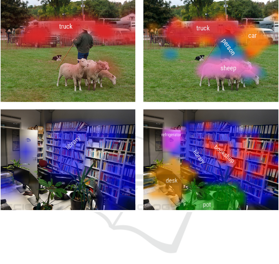
(a) CAM (b) DCM

Figure 1: Exemplary comparison of localization results obtained with CAMs (left) and our DCMs (right). The upper example

is from the MS COCO dataset (Lin et al., 2014) and both ResNet-50 models were trained on cropped instances from COCO.

The lower example shows a photo of our ofﬁce and uses models trained on ImageNet-1k (Russakovsky et al., 2015).

jective allow us to choose a constant global thresh-

old across all classes for determining whether an ob-

ject is present at each location in the feature map and

what type of object it is. The resulting dense class

map (DCM) resembles a coarse semantic segmenta-

tion. Fig. 1 illustrates this with two examples. Even

though the network has only been trained to assign

a single class label to an entire image as a whole,

it can be modiﬁed to locate a variety of objects in a

complex scene. We describe our approach in detail in

Section 3, after brieﬂy reviewing CAMs Section 2.

In Section 4, we present quantitative and qualita-

tive experimental results on the ILSVRC 2012 Local-

ization Challenge (Russakovsky et al., 2015) and the

MS COCO object detection task (Lin et al., 2014).

We ﬁnd that DCMs match the performance of CAMs

if the image only contains a single dominant object to

be localized, but largely outperform them for detect-

ing multiple objects in a single scene.

Finally, we outline related work in Section 5 and

summarize our conclusions in Section 6.

2 BACKGROUND: CAMS

Class activation maps (CAMs) have been introduced

by Zhou et al. (2016) as a technique for enhanc-

ing a CNN pre-trained for image-level classiﬁcation

with object localization capabilities after the training.

Since our dence class maps (DCMs) build up on this

approach, we brieﬂy review CAMs in the following.

Let ψ : R

H ×W ×3

→ R

×W

×D

denote a feature

extractor realized by a CNN up to the last convolu-

tional layer. Given an image with height H and width

W , ψ computes a spatial feature map consisting of

× W

local feature vectors of dimensionality D.

Due to pooling, the size of this feature map is typi-

cally only a fraction of the original image size.

VISAPP 2022 - 17th International Conference on Computer Vision Theory and Applications

288

In most modern CNN architectures, e.g., ResNet

(He et al., 2016), these local feature cells are averaged

into a single feature vector, which is passed through a

classiﬁcation layer with weight matrix W ∈ R

C×D

and

bias vector b ∈ R

, where C denotes the number of

classes. The resulting class scores are ﬁnally mapped

into the space of probability distributions using the

softmax activation function:

softmax(y)

exp(y

)

∑

j=1

exp(y

)

. (1)

Formally, the predicted probabilities for an input im-

age x are obtained as:

f (x) = softmax

W ·

∑

i, j

ψ(x)

i, j

· W

+ b

. (2)

The key insight of Zhou et al. (2016) is that, due to

linearity, the classiﬁer can also be applied to each lo-

cal feature cell before pooling without changing the

result:

f (x) = softmax

∑

i, j

W · ψ(x)

i, j

+ b

· W

. (3)

The predicted global logits are hence the average of

region-wise class scores. These local scores for any

c ∈ {1, . .. ,C} are the class activation map of class c:

CAM(x)

i, j,c

= W

· ψ(x)

i, j

+ b

. (4)

Even though the classiﬁer has only been trained on

image-wise labels, Zhou et al. (2016) found that the

CAM of the top-scoring class can effectively localize

instances of that class. To this end, they threshold the

CAM by 20% of its maximum and draw a bounding

box around the largest connected component.

3 METHOD

3.1 Cosine Loss

The relative thresholding approach of CAMs hints at

one of their main issues: Before the softmax activa-

tion, the ranges of the CAMs for different classes are

usually not comparable. This complicates setting a

single threshold for deciding whether a certain object

is present at a given location in the image or not (see

Fig. 2a). If the softmax activation would be applied—

which CAMs do not—distinguishing between objects

and noisy background patches became an issue, since

these could reach similarly high activation values due

to the softmax operation (see Figs. 2c and 2e).

These problems do not exist when using the co-

sine loss (Barz and Denzler, 2020) for training, which

enables us to use a single absolute threshold for the si-

multaneous detection of multiple classes instead of a

single one. Instead of the softmax function, the cosine

loss applies L

normalization to the feature represen-

tation ˆx ∈ R

of the input computed by the network

and maximizes its cosine similarity to the embedding

ϕ(c) of the ground-truth class c ∈ {1, . . . ,C}:

cos

( ˆx,c)

= 1 −

h ˆx, ϕ(c) i

k ˆxk· kϕ(c)k

. (5)

The class embeddings ϕ(c) can be derived from prior

semantic knowledge such as class taxonomies (Barz

and Denzler, 2019), from world knowledge encoded

in large text corpora (Frome et al., 2013), or simply

be one-hot encodings. In the latter case, the cosine

loss maximizes the c-th entry of the prediction vector

after L

normalization. Compared to cross-entropy

with softmax, it enforces this channel less strictly to

become 1.

It can be seen in Fig. 2d that foreground and back-

ground are much better separated in the histogram of

maximum class scores after applying the activation.

The L

normalization also accounts for making the re-

sponses at different locations comparable by discard-

ing the magnitude of the difference between predicted

features and class embeddings and focusing on their

angle instead.

3.2 Dense Class Maps

Leveraging these advantages of the cosine loss, we

build upon the idea of CAMs and obtain a dense map

of class embeddings DCE : R

H ×W ×3

→ R

×W

×D

for an image x ∈ R

H ×W ×3

by removing the global

average pooling layer and converting the embedding

layer with weights W ∈ R

×D

and biases b ∈ R

into

a 1 × 1 convolution. The entire procedure is depicted

schematically in Fig. 3.

In contrast to CAMs, which do not apply the soft-

max activation on the local predictions, we apply the

normalization at each cell of the resulting tensor:

DCE(x)

i, j

W · ψ(x)

i, j

+ b

kW · ψ(x)

i, j

+ bk

. (6)

Averaging over all locations of the resulting dense

embedding maps is, hence, not equivalent anymore

to the output of the original network.

We can then assign a label class(x, i, j) ∈

{1, . . .,C} to each local cell by ﬁnding the class em-

bedding that is most similar to its local feature vector:

sim(x, i, j, c) = h DCE(x)

i, j

, ϕ(c) i, (7a)

class(x, i, j) = argmax

c=1,...,C

sim(x, i, j, c). (7b)

Weakly-supervised Localization of Multiple Objects in Images using Cosine Loss

289

(a)

Before Activation

Trained with Cross-Entropy

0 50

(b)

Trained with Cosine Loss

0 100

100

125

150

(c)

After Activation

0.0 0.5 1.0

(d)

0.0 0.5 1.0

100

(e)

After Thresholding

0.0 0.5 1.0

100

120

140

(f)

0.0 0.5 1.0

100

120

140

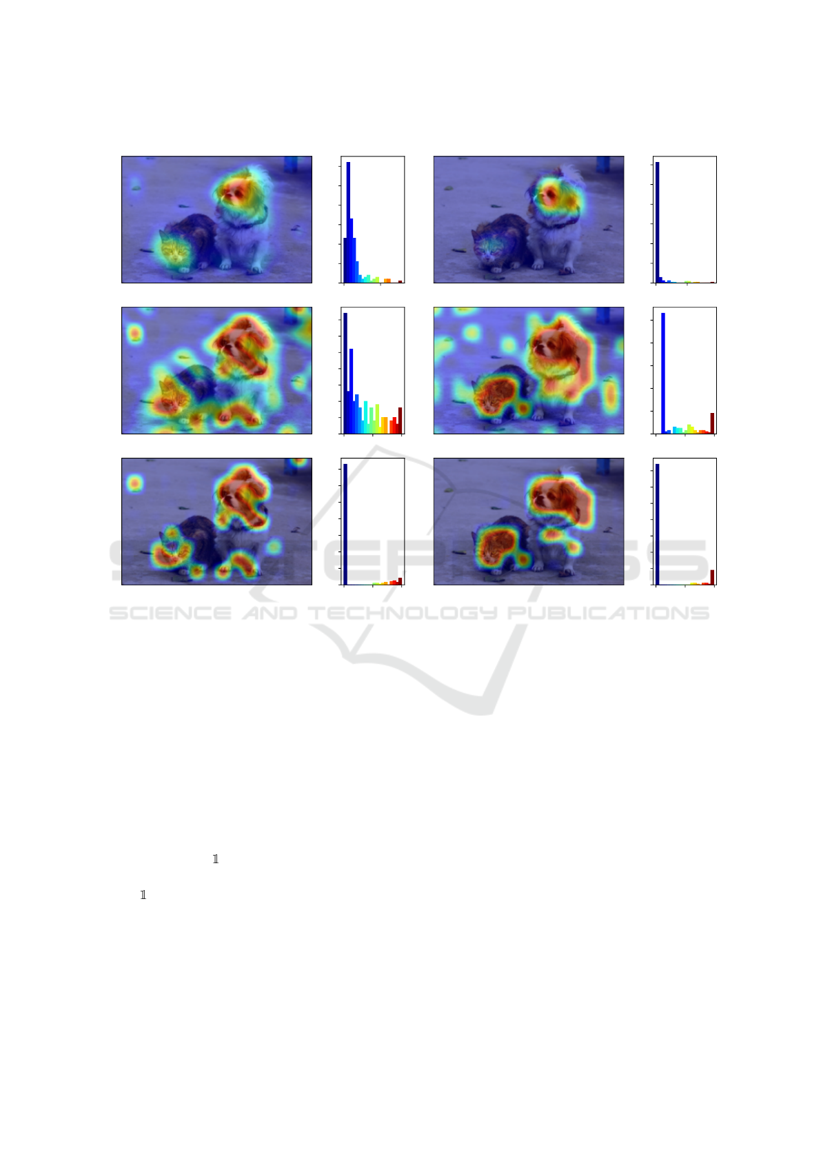
Figure 2: Heatmaps and histograms of the maximum value over all classes at each cell of a DCM, before and after the

activation. The activation function is softmax for the cross-entropy loss and L

normalization for the cosine loss. The hyper-

parameters for thresholding are ϑ

cls

= 0.8, ϑ

sim

= 0.5.

However, many of these cells will contain back-

ground, such that assigning an object class to them

is not reasonable and the results will be noisy. Thus,

we ﬁrst determine a set C(x) ⊆ {1, . . . ,C} of classes

that are present in the image by assigning a score to

each class and selecting those classes whose score

is greater than a certain threshold ϑ

cls

∈ [0, 1], i.e.,

C(x) = {c ∈ {1, .. . ,C}|score(x, c) > ϑ

cls

}. The score

for a given class is deﬁned as the maximum cosine

similarity to its class embedding over all locations to

which this class has been assigned:

score(x, c) = max

i, j

{class(x,i, j)=c}

· sim(x, i, j, c), (8)

where

{·}

is the indicator function, being one if the

argument evaluates to true and zero otherwise. This

scoring procedure is different from simply selecting

the globally top-scoring classes, since two related

classes could obtain high scores at identical positions.

With our approach, only the highest-scoring of such

overlapping classes will be selected.

For ﬁnding the locations where the selected

classes are present, we threshold their cosine simi-

larity with a second threshold ϑ

sim

≤ ϑ

cls

to obtain

a dense class map DCM(x, i, j) ∈ {0, 1, . . . ,C}, where

0 denotes the background class:

DCM(x, i, j) =







class(x, i, j) if class(x, i, j) ∈ C and

sim(x, i, j, class(x, i, j)) > ϑ

sim

0 else.

(9)

An example of the similarity scores corresponding to

the resulting class maps after this two-stage thresh-

olding procedure—ﬁrst across classes, then across

locations—is given in Fig. 2f. The actual output that

is relevant for practical use, however, is the hard as-

signment of locations to classes given by the DCM.

This can be visualized by color-coding classes as done

in Fig. 1.

VISAPP 2022 - 17th International Conference on Computer Vision Theory and Applications

290

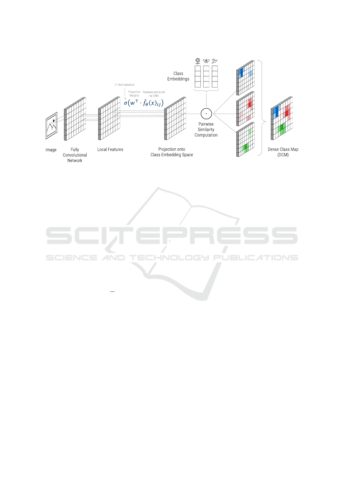
Figure 3: Schematic illustration of the pipeline for computing a dense class map.

3.3 Implementation Details

While training images annotated with a single class

usually show a close-up of the object of interest,

we are interested in analyzing more complex scenes

where the objects are smaller. Thus, we use a higher

input image resolution for generating DCMs than the

resolution typically used for training the network,

which usually is 224 × 224 for a ResNet trained on

ImageNet (He et al., 2016). For dense classiﬁcation,

we resize the input images so that their larger side is

640 pixels wide.

It is worth noting that the resolution of the fea-

ture map obtained from the last convolutional layer,

and hence the resolution of the DCM as well, is rather

coarse. In the case of the ResNet-50 architecture, the

dimensions of the DCM are

of the original image

dimensions. For visualization purposes, we upsample

the DCM and all heatmaps to the size of the image

using bicubic interpolation, which results in a rather

blurry semantic segmentation.

For generating bounding boxes instead of segmen-

tations, we generate one box for each class in C fol-

lowing the approach of Zhou et al. (2016): The simi-

larity map sim(x, ·, ·, c) for class c ∈ C is thresholded

with ϑ

bbox

· max

i, j

sim(x, i, j, c), where ϑ

bbox

∈ [0, 1],

and a box is drawn around the largest connected com-

ponent.

4 EXPERIMENTS

We evaluate our DCM approach in comparison to

CAMs in two settings: First, we conduct WSL on

the ImageNet-1k dataset (Russakovsky et al., 2015),

which mainly comprises images showing a single

dominant object and provides a single class label and

corresponding bounding box per image. This exper-

iment serves as a veriﬁcation that DCMs do not per-

form worse than CAMs in this restricted setting, in

which CAMs typically operate. Second, we use the

MS COCO dataset (Lin et al., 2014), an established

benchmark for object detection, for evaluating both

approaches in a more realistic setting where multiple

different classes are present in a single image.

4.1 Semantic Information

As mentioned in Section 3.1, using the cosine loss for

training allows for straightforward integration of prior

knowledge in the form of semantic class embeddings.

In addition to one-hot encodings, we evaluate DCMs

on networks trained with the hierarchy-based seman-

tic embeddings proposed by Barz and Denzler (2019).

These embeddings are constructed so that their pair-

wise cosine similarity equals a semantic similarity

measure derived from a class taxonomy.

To obtain such a taxonomy covering the 80 classes

of MS COCO, we map them manually to matching

synsets from the WordNet ontology (Fellbaum, 1998).

However, the WordNet graph is not a tree, because

some concepts have multiple parent nodes. Thus, we

prune the subgraph of WordNet in question to a tree

using the approach of Redmon and Farhadi (2017):

We start with a tree consisting of the paths from the

root to all classes from MS COCO which have only

one such root path. Then, the remaining classes are

added successively by choosing that path among their

several root paths that results in the least number of

nodes added to the existing tree.

Weakly-supervised Localization of Multiple Objects in Images using Cosine Loss

291

4.2 Training Details

For all our experiments, we train a ResNet-50 (He

et al., 2016) using stochastic gradient descent with

a cyclic learning rate schedule with warm restarts

(Loshchilov and Hutter, 2017). The base cycle length

is 12 epochs and is doubled after each cycle. We

use ﬁve cycles, amounting to a total of 372 training

epochs. The base learning rate is 0.1.

For training on ImageNet-1k, the model is initial-

ized with random weights. These pre-trained weights

are used as initialization for training on MS COCO.

Since our training objective is single-label classi-

ﬁcation but images in MS COCO typically contain

multiple objects, we extract crops of each individual

object using the provided bounding box annotations,

ignoring small objects whose bounding box is smaller

than 32 pixels in both dimensions. As a result, we ob-

tain 684,070 training images of object instances.

To present the CNN with objects of various scales

as well as truncated objects during training, we re-

size the training images by choosing the target size of

their smaller side from [256, 480] at random and ex-

tract a square crop of size 224×224. We furthermore

use random horizontal ﬂipping and random erasing

(Zhong et al., 2017) as data augmentation.

4.3 WSL on ImageNet-1k

As a sanity check, we ﬁrst evaluate the localization

performance of DCMs on the easier task of locating

a single predominant object in an image using the

ImageNet-1k dataset. Following the evaluation pro-

tocol deﬁned for the ImageNet Large Scale Recogni-

tion Challenge (ILSVRC) 2012 (Russakovsky et al.,

2015), we assess performance in terms of the average

top-5 localization error. For a single image, the er-

ror is 0 if at least one of the top-5 predicted bounding

boxes belongs to the object class assigned to the im-

age and has at least 50% overlap with the ground-truth

bounding box of that object. Otherwise, the error is 1.

We obtain the same top-5 localization error of

48% with both CAMs applied to a CNN trained

with cross-entropy and with DCMs applied to a

CNN trained with the cosine loss and one-hot encod-

ings. For CAMs, this performance was obtained with

bbox

= 0.2, while we used ϑ

bbox

= 0.06 for DCMs.

Zhou et al. (2016) used different network architec-

tures for their CAM experiments, but the performance

reported by them is similar.

Thus, both approaches perform equally well on

the object localization task of ILSVRC 2012. This

was expected, since ILSVRC is easy in this regard.

Most images contain only a single object, which often

even ﬁlls a large part of the image. Detecting multi-

ple objects from different classes and of smaller size

is hence not necessary in this scenario.

4.4 WSL on MS COCO

4.4.1 Evaluation Metric

The MS COCO dataset poses a much more difﬁ-

cult challenge for WSL by presenting a real detec-

tion task. Performance is hence typically evaluated

in terms of mean average precision (mAP). COCO

uses an average over 20 mAP values with differ-

ent intersection-over-union (IoU) thresholds varying

from 50% to 95%. In this work, however, we are

not dealing with a fully supervised scenario and the

WSL methods never see ideal bounding boxes during

training. Therefore, the predicted bounding box can

in many cases be much smaller than the ground-truth

bounding box if only a single characteristic part of the

object is used for the classiﬁcation decision (e.g., only

the head of a dog instead of the entire body). On the

other hand, it can also be larger if many objects of the

same class stand close together.

These predictions can, however, still be helpful for

determining which objects are located where in the

image, even if the localization is not highly accurate.

Therefore, we report mAP with a more relaxed IoU

threshold of 25%. In addition, we also compute mAP

with an IoU threshold of 0%, which does not require

any overlap with the ground-truth bounding box at all

and hence evaluates multi-label classiﬁcation perfor-

mance, where we are only interested in which objects

are present in the image, but not where they are.

4.4.2 Bounding Box Hyper-parameters

Since average precision summarizes the performance

of a detector over all possible detection thresholds, we

do not need to ﬁx the class score threshold ϑ

cls

for this

experiment. The bounding box generation threshold,

on the other hand, is tuned on the uncropped train-

ing set individually for each method and then applied

on the test set for the ﬁnal performance evaluation.

This results in ϑ

bbox

= 0.25 for CAMs, ϑ

bbox

= 0.3

for DCMs with one-hot encodings, and ϑ

bbox

= 0.75

for DCMs with semantic class embeddings. The com-

paratively high threshold in the latter case has an in-

tuitive explanation, since different objects are consid-

ered more similar to each other on average with se-

mantic embeddings than with one-hot encodings, re-

quiring a higher threshold to prevent over-detection.

VISAPP 2022 - 17th International Conference on Computer Vision Theory and Applications

292

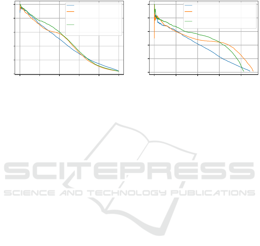
(a) IoU threshold 0%

0.0 0.2 0.4 0.6 0.8 1.0

Recall

0.0

0.2

0.4

0.6

0.8

1.0

Precision

Cross-Entropy [AP: 43.0%]

Cosine Loss + One-hot

Encodings + DCM

[AP: 43.3%]

Cosine Loss + Semantic

Embeddings + DCM

[AP: 46.1%]

(b) IoU threshold 25%

0.0 0.1 0.2 0.3 0.4

Recall

0.0

0.2

0.4

0.6

0.8

1.0

Precision

Cross-Entropy + CAM [AP: 17.0%]

Cosine Loss + One-hot Encodings

+ DCM [AP: 21.6%]

Cosine Loss + Semantic Embeddings

+ DCM [AP: 21.8%]

Figure 4: Precision-recall curves for CAMs and DCMs on MS COCO with IoU thresholds of 0% and 25%.

4.4.3 Results

Precision-recall curves and the mAP obtained on the

test set are presented in Fig. 4. First, it can be seen that

even for the task of multi-label classiﬁcation with-

out localization (Fig. 4a), the cosine loss combined

with DCMs improves mAP slightly compared to net-

works trained with cross-entropy (43.3% vs. 43.0%).

Apparently, suppressing non-maximum class predic-

tions at identical locations—as done by DCMs—

helps avoiding false positive predictions. Integrating

prior semantic knowledge in the form of hierarchy-

based class embeddings improves mAP much further

by three percent points.

The differences are more pronounced, though, in

an actual object detection setting, as can be seen in

Fig. 4b. Using the cosine loss and DCMs allows for

maintaining a much higher precision when lowering

the detection threshold: For a recall level of 30%, the

precision of DCMs with semantic embeddings or one-

hot encodings is still 44%, while CAMs applied to

a CNN trained with cross-entropy only obtain 23%

precision at this level of recall.

As before, semantic embeddings surpass one-hot

encodings. They do not obtain the same maximum

recall, but provide better precision, i.e., less false pos-

itives, for most recall levels. But even without se-

mantic embeddings, DCMs outperform CAMs by a

relative increase of 27% mAP.

4.5 Qualitative Examples

Two qualitative examples comparing CAMs and

DCMs on ImageNet-1k and MS COCO are shown in

Fig. 1. Further examples from MS COCO including

bounding boxes are presented in Fig. 5.

For CAMs, we consider all classes with a pre-

dicted probability of at least 15% to be present in

the image, since second-best predictions often have

low scores due to the softmax operation. Regarding

DCMs, we want to select only those classes whose

embeddings are highly similar to at least one local

feature and hence use the threshold ϑ

cls

= 0.99. To

obtain the coarse semantic segmentations, we set the

threshold applied to the similarity maps of selected

classes equal to the one used for bounding box gen-

eration, i.e., ϑ

sim

= ϑ

bbox

, using the bounding box

thresholds given above.

The ﬁrst example in Fig. 5 shows an image com-

prising objects from two different classes. CAMs are

only able to detect one of these correctly due to the

strong decision enforced by the softmax activation.

The use of the cosine loss and DCMs, on the other

hand, allows us to detect both objects in the image us-

ing a global threshold across all classes based on the

cosine similarity between the predicted features and

the class embeddings.

Additionally, integrating prior knowledge about

the similarity between classes and hence not forcing

the network to consider cars and trucks as two com-

pletely different things allows the DCM to also pro-

vide the correct prediction “car” along with “truck”,

even though the latter has a slightly higher score.

Thanks to semantic embeddings, both classes can

have high scores simultaneously, since they are se-

mantically similar. Due to the reduced competition

between them, not only “truck” exceeds the threshold

cls

, but “car” can do so too.

The second example shows a more complex scene,

where DCMs, especially with semantic embeddings,

are able to detect substantially more objects than

CAMs. They do not only detect the train and the

bench but also the bicycle, the table, and the person.

Weakly-supervised Localization of Multiple Objects in Images using Cosine Loss

293

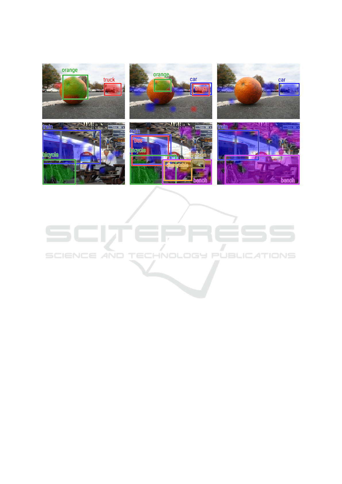
(a) DCM (one-hot) (b) DCM (semantic) (c) CAM

Figure 5: Qualitative examples from MS COCO with bounding boxes.

5 RELATED WORK

5.1 Class Activation Maps

The applicability of CAMs is restricted by design to

CNN architectures with global average pooling fol-

lowed by a single classiﬁcation layer. Grad-CAM

(Selvaraju et al., 2017) is a generalization of CAMs,

which determines weights for the different channels

of the convolutional feature map based on the gradient

of the network output with respect to the activations

in each channel. This allows for obtaining activation

maps for arbitrary CNN architectures as well as net-

works trained for a task different from classiﬁcation,

such as image captioning or question answering.

Gradient-based methods exhibit some drawbacks,

though, such as being strongly inﬂuenced by the input

image and less sensitive to the actual model (Adebayo

et al., 2018). Desai and Ramaswamy (2020) avoid

these issues by proposing a gradient-free variant of

CAMs based on an ablation procedure. This so-called

Ablation-CAM determines the weights for the feature

channels based on the change of the model output if

this channel would be set to zero.

These modiﬁcations of the original CAM tech-

nique make it more widely applicable to different

types of models but do not entail signiﬁcant advan-

tages over the localization performance of CAMs for

ResNet-like classiﬁers. Most notably, they do not ad-

dress the limitation of not being able to detect more

than one class per image, which we focus on.

5.2 Weakly-supervised Localization

Other common issues of CAMs are under- and over-

detection: For some classes, CAMs focus only on the

most salient parts of the object and ignore the rest,

e.g., the heads of persons instead of their body, result-

ing in too small bounding boxes. Concerning certain

other classes such as trains, for example, the classi-

ﬁer often considers context features like rails to be

indicative of the object, such that they are mistakenly

included in the bounding box.

The latter problem is tackled by soft proposal net-

works (SPNs) (Zhu et al., 2017), which mask the com-

puted feature map with soft objectness scores that

are obtained by a random walk on a fully-connected

graph over all cells of the feature map. The edge

weights of the graph depend on feature differences

and spatial distance, such that high objectness scores

are assigned to cells that are highly different from

their neighbors. These masks are intended to cast a

spotlight onto the actual object, reducing the inﬂuence

of the context. Since the object proposals depend di-

rectly on the feature map itself, they are trained jointly

with the network.

To mitigate the problem of under-detection, Du-

rand et al. (2017) learn and average multiple CAMs

per class. While they intend these maps to high-

light different object parts such as heads, legs etc.,

this property is not explicitly enforced. Zhang et al.

(2018) employ a two-branch classiﬁer and use the

CAM obtained from the ﬁrst classiﬁer to erase the

VISAPP 2022 - 17th International Conference on Computer Vision Theory and Applications

294

respective object parts from the feature map before

passing it through the second classiﬁer, so that this

one is forced to focus on different characteristic fea-

tures of the object. At inference time, the two CAMs

are aggregated by taking the element-wise maximum.

As opposed to these approaches, which modify

the network architecture with the goal of improving

the localization accuracy of CAMs, we do not explic-

itly aim for improving the state of the art in WSL of

single objects. In fact, a recent study found that no

WSL method proposed after CAMs actually outper-

form them in a realistic setting for segmenting images

into foreground and background (Choe et al., 2020).

In our work, we extend the WSL approach in-

spired by CAMs for detecting multiple classes at once

without needing to tailor the network architecture or

learning process to this task. Instead, we ﬁnd that

the simple change of the loss function to the cosine

loss for classiﬁer pre-training facilitates generating a

joint activation map for all classes present in the im-

age without additional cost.

5.3 Cosine Loss

The cosine loss mainly enjoys popularity in the area

of multi-modal representation learning and cross-

modal retrieval (Sudholt and Fink, 2017; Salvador

et al., 2017), where it is used for maximizing the

similarity between embeddings of two related sam-

ples from different modalities (e.g., images and cap-

tions). Similar to aligning representations for differ-

ent modalities, it has also proven useful for match-

ing learned image representations with semantic class

embeddings for semantic image retrieval (Barz and

Denzler, 2019). Qin et al. (2008) furthermore used the

cosine loss for a list-wise learning to rank approach,

where a vector of predicted ranking scores is com-

pared to a vector of ground-truth scores using the co-

sine similarity.

Barz and Denzler (2020) recently proposed to

employ the cosine loss for classiﬁcation either as a

replacement for or in combination with the cross-

entropy loss. They found that the L

normalization

applied by the cosine loss acts as a useful regularizer

that improves the classiﬁcation performance when

few training data is available. We follow their work in

the sense that we also train CNN classiﬁers using the

cosine loss, but we study the properties of the learned

representations from a different perspective, i.e., their

advantages for weakly-supervised localization.

6 CONCLUSIONS

We proposed an extension of the popular class ac-

tivation maps (CAMs) for weakly-supervised local-

ization of multiple classes in images. The basis of

our approach is the use of the cosine loss instead of

cross-entropy with softmax for training the classiﬁer

on images of individual objects. We found the sim-

ilarities between local feature cells and class embed-

dings to be better comparable across different classes

than class prediction scores generated by softmax net-

works, which allows for detecting the presence of

multiple classes using a ﬁxed global threshold.

Experiments on the MS COCO dataset showed

that our dense class maps (DCMs) improve the object

detection performance compared to CAMs by a rela-

tive amount of 27% mAP with one-hot encodings and

by 28% with semantic class embeddings. At a recall

level of 30%, DCMs provide almost twice the preci-

sion of CAMs. With semantic embeddings, DCMs do

not achieve the same maximum recall as with one-hot

encodings, but maintain higher precision.

Even in the easier scenario of multi-label classi-

ﬁcation without localization, DCMs provide a 0.7%

better accuracy. Adding prior knowledge in the form

of semantic class embeddings improves the accuracy

much further by another 6%.

So far, we relied on the property that images in

the dataset used for classiﬁcation pre-training dis-

play a single dominant object. Future work might

explore approaches for extending the cosine loss to

multi-label classiﬁcation, so that the pre-training with

image-level class labels can be conducted on more

generic and complex images.

REFERENCES

Adebayo, J., Gilmer, J., Muelly, M., Goodfellow, I., Hardt,

M., and Kim, B. (2018). Sanity checks for saliency

maps. In Bengio, S., Wallach, H., Larochelle, H.,

Grauman, K., Cesa-Bianchi, N., and Garnett, R., edi-

tors, Advances in Neural Information Processing Sys-

tems (NeurIPS), volume 31. Curran Associates, Inc.

Barz, B. and Denzler, J. (2019). Hierarchy-based image

embeddings for semantic image retrieval. In IEEE

Winter Conference on Applications of Computer Vi-

sion (WACV), pages 638–647.

Barz, B. and Denzler, J. (2020). Deep learning on small

datasets without pre-training using cosine loss. In

IEEE Winter Conference on Applications of Computer

Vision (WACV), pages 1360–1369.

Choe, J., Oh, S. J., Lee, S., Chun, S., Akata, Z., and Shim,

H. (2020). Evaluating weakly supervised object local-

ization methods right. In IEEE Conference on Com-

Weakly-supervised Localization of Multiple Objects in Images using Cosine Loss

295

puter Vision and Pattern Recognition (CVPR), pages

3130–3139.

Desai, S. and Ramaswamy, H. G. (2020). Ablation-CAM:

Visual explanations for deep convolutional network

via gradient-free localization. In IEEE Winter Con-

ference on Applications of Computer Vision (WACV),

pages 972–980.

Durand, T., Mordan, T., Thome, N., and Cord, M. (2017).

WILDCAT: Weakly supervised learning of deep con-

vnets for image classiﬁcation, pointwise localization

and segmentation. In IEEE Conference on Computer

Vision and Pattern Recognition (CVPR), pages 5957–

5966.

Fellbaum, C. (1998). WordNet. Wiley Online Library.

Frome, A., Corrado, G. S., Shlens, J., Bengio, S., Dean,

J., Ranzato, M., and Mikolov, T. (2013). DeViSE: A

deep visual-semantic embedding model. In Interna-

tional Conference on Neural Information Processing

Systems (NIPS), NIPS’13, pages 2121–2129, USA.

Curran Associates Inc.

He, K., Zhang, X., Ren, S., and Sun, J. (2016). Deep

residual learning for image recognition. In IEEE Con-

ference on Computer Vision and Pattern Recognition

(CVPR), pages 770–778.

Kuznetsova, A., Rom, H., Alldrin, N., Uijlings, J., Krasin,

I., Pont-Tuset, J., Kamali, S., Popov, S., Malloci, M.,

Kolesnikov, A., Duerig, T., and Ferrari, V. (2020).

The open images dataset v4: Uniﬁed image classiﬁ-

cation, object detection, and visual relationship detec-

tion at scale. International Journal of Computer Vi-

sion (IJCV).

Lin, T.-Y., Maire, M., Belongie, S., Hays, J., Perona, P., Ra-

manan, D., Doll

ar, P., and Zitnick, C. L. (2014). Mi-

crosoft COCO: Common objects in context. In Fleet,

D., Pajdla, T., Schiele, B., and Tuytelaars, T., editors,

European Conference on Computer Vision (ECCV),

pages 740–755, Cham. Springer International Pub-

lishing.

Loshchilov, I. and Hutter, F. (2017). SGDR: Stochastic

gradient descent with warm restarts. In International

Conference on Learning Representations (ICLR).

Qin, T., Zhang, X.-D., Tsai, M.-F., Wang, D.-S., Liu, T.-

Y., and Li, H. (2008). Query-level loss functions for

information retrieval. Information Processing & Man-

agement, 44(2):838–855.

Redmon, J. and Farhadi, A. (2017). YOLO9000: Better,

faster, stronger. In IEEE Conference on Computer Vi-

sion and Pattern Recognition (CVPR), pages 6517–

6525.

Russakovsky, O., Deng, J., Su, H., Krause, J., Satheesh, S.,

Ma, S., Huang, Z., Karpathy, A., Khosla, A., Bern-

stein, M., Berg, A. C., and Fei-Fei, L. (2015). Im-

agenet large scale visual recognition challenge. In-

ternational Journal of Computer Vision, 115(3):211–

252.

Salvador, A., Hynes, N., Aytar, Y., Marin, J., Oﬂi, F., We-

ber, I., and Torralba, A. (2017). Learning cross-modal

embeddings for cooking recipes and food images. In

IEEE Conference on Computer Vision and Pattern

Recognition (CVPR), pages 3068–3076. IEEE.

Selvaraju, R. R., Cogswell, M., Das, A., Vedantam, R.,

Parikh, D., and Batra, D. (2017). Grad-CAM: Visual

explanations from deep networks via gradient-based

localization. In IEEE International Conference on

Computer Vision (ICCV), pages 618–626.

Sudholt, S. and Fink, G. A. (2017). Evaluating word string

embeddings and loss functions for CNN-based word

spotting. In International Conference on Document

Analysis and Recognition (ICDAR), volume 1, pages

493–498. IEEE.

Sun, C., Shrivastava, A., Singh, S., and Gupta, A. (2017).

Revisiting unreasonable effectiveness of data in deep

learning era. In IEEE International Conference on

Computer Vision (ICCV).

Wu, B., Chen, W., Fan, Y., Zhang, Y., Hou, J., Liu, J., and

Zhang, T. (2019). Tencent ML-images: A large-scale

multi-label image database for visual representation

learning. IEEE Access, 7:172683–172693.

Zhang, X., Wei, Y., Feng, J., Yang, Y., and Huang,

T. S. (2018). Adversarial complementary learning for

weakly supervised object localization. In IEEE Con-

ference on Computer Vision and Pattern Recognition

(CVPR), pages 1325–1334.

Zhong, Z., Zheng, L., Kang, G., Li, S., and Yang, Y. (2017).

Random erasing data augmentation. arXiv preprint

arXiv:1708.04896.

Zhou, B., Khosla, A., Lapedriza, A., Oliva, A., and Tor-

ralba, A. (2016). Learning deep features for discrimi-

native localization. In IEEE Conference on Computer

Vision and Pattern Recognition (CVPR), pages 2921–

2929.

Zhu, Y., Zhou, Y., Ye, Q., Qiu, Q., and Jiao, J. (2017). Soft

proposal networks for weakly supervised object local-

ization. In IEEE International Conference on Com-

puter Vision (ICCV), pages 1859–1868.

VISAPP 2022 - 17th International Conference on Computer Vision Theory and Applications

296