Solving Large Steiner Tree Problems in Graphs for Cost-efficient
Fiber-To-The-Home Network Expansion
Tobias M
¨
uller
1
, Kyrill Schmid
1
, Dani
¨
elle Schuman
1
, Thomas Gabor
1
, Markus Friedrich
1
and Marc Geitz
2
1
Mobile and Distributed Systems Group, LMU Munich, Germany
2
Telekom Innovation Laboratories, Deutsche Telekom AG, Bonn, Germany
Keywords:
Network Planning, FTTH, Evolutionary Algorithm, Simulated Annealing, Quantum Computing, Physarum,
Steiner Tree Problem, Optimization.
Abstract:
The expansion of Fiber-To-The-Home (FTTH) networks creates high costs due to expensive excavation pro-
cedures. Optimizing the planning process and minimizing the cost of the earth excavation work therefore lead
to large savings. Mathematically, the FTTH network problem can be described as a minimum Steiner Tree
problem. Even though the Steiner Tree problem has already been investigated intensively in the last decades,
it might be further optimized with the help of new computing paradigms and emerging approaches. This work
studies upcoming technologies, such as Quantum Annealing, Simulated Annealing and nature-inspired meth-
ods like Evolutionary Algorithms or slime-mold-based optimization. Additionally, we investigate partitioning
and simplifying methods. Evaluated on several real-life problem instances, we could outperform a traditional,
widely-used baseline (NetworkX Approximate Solver (Hagberg et al., 2008)) on most of the domains. Prior
partitioning of the initial graph and the slime-mold-based approach were especially valuable for a cost-efficient
approximation. Quantum Annealing seems promising, but was limited by the number of available qubits.
1 INTRODUCTION
Internet traffic is constantly increasing over time
due to growing digitization and the increasing use
of bandwidth intensive applications. Internet con-
sumers, be it large industry, small enterprises or pri-
vate households require glass fiber (FTTH) connec-
tion to meet the increasing demand. The main cost
driver of fiber roll-out for land lines is the earth ex-
cavation cost. Optimizing the planning process and
finding better networks can reduce needed excavation,
which leads to large savings. Figure 1 visualizes an
exemplary cadastral excerpt with house connections
and access nodes for which an optimal network needs
to be found with respect to the ditch cost map on the
right.
Finding a cost-minimal solution for connecting
multiple FTTH households can be described as a
Steiner Tree Problem (Pr
¨
omel and Steger, 2012).
Calculating minimum Steiner Trees is a well-known
problem and has already been investigated in a vari-
ety of network approximation use cases (Gupta and
K
¨
onemann, 2011). However, the emergence of new
computing paradigms and novel approaches opens up
new possibilities to tackle the Steiner Tree problem.
This work has the goal to analyse emerging so-
lution methods such as nature inspired algorithms
and Quantum Annealing technologies to find opti-
mal network configurations for a given problem in-
stance. Since we want to solve real-life problems, we
focused on developing a practical, easy-to-use appli-
cation. Therefore, we implemented a Python-based
demonstrator, where cadaster data can be easily im-
ported and transformed into a corresponding Steiner
Tree problem. We implemented various methods to
solve, simplify and partition the resulting graph.
We chose nature-inspired solution methods, such
as an Evolutionary Algorithm (EA) (Rosenberg et al.,
2021) or a Physarum solver based on the behav-
ior of the Physarum polycephalum slime mold (Sun,
2019). We also included a Simulated Annealing (SA)
algorithm which finds solutions by building a long
Markov Chain (Kapsalis et al., 1993b) and a Quantum
Annealing (QA) solver based on a Quadratic Uncon-
strained Binary Optimization (QUBO) formulation of
the Steiner Tree problem (Lucas, 2014).
Müller, T., Schmid, K., Schuman, D., Gabor, T., Friedrich, M. and Geitz, M.
Solving Large Steiner Tree Problems in Graphs for Cost-efficient Fiber-To-The-Home Network Expansion.
DOI: 10.5220/0010749300003116
In Proceedings of the 14th International Conference on Agents and Artificial Intelligence (ICAART 2022) - Volume 3, pages 23-32
ISBN: 978-989-758-547-0; ISSN: 2184-433X
Copyright
c
 2022 by SCITEPRESS – Science and Technology Publications, Lda. All rights reserved
23

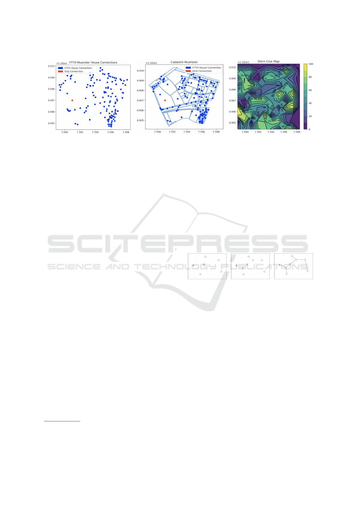
(a) Grid and House Connections (b) Connections and Streets (c) Ditch Cost Map
Figure 1: Example of a cadastral excerpt (Figure 1a) with mapped FTTH house connections (blue) and access nodes (red).
Figure 1b additionally displays street courses. The ditch cost map (Figure 1c) provides the excavation costs per meter.
These different solution methods have been com-
pared and evaluated against a commonly known base-
line (NetworkX approximated Steiner Tree solver
1
).
For larger instances the solvers mentioned above may
become intractable due to the exponential increase in
complexity. Therefore, we also provide methods to
simplify or partition a given problem and run solvers
on the simplified (respectively partitioned) graph. Af-
ter a simplifier or partitioner has been applied, the
problem can be passed again into a solver method,
thereby decreasing the duration of the optimization
significantly.
Summarized, our contributions are two-fold:
• We provide a wide range of state-of-the-art al-
gorithms for solving, simplifying and partition-
ing large Steiner Tree problems in graphs. These
methods are comprised in a demonstrator.
• We provide a thorough evaluation of these meth-
ods on real-world problems and their impacts on
resulting network costs and runtime.
2 PRELIMINARIES
2.1 The Steiner Tree Problem
Formally, the problem of finding a cost-minimal net-
work to connect N FTTH house connections with M
access nodes can be described as a Steiner Tree Prob-
lem (STP) (Pr
¨
omel and Steger, 2012). The formula-
tion of the STP is defined as follows. Let G be an
undirected weighted graph G = (V,E), with V as the
set of nodes and E as the set of edges. The set of nodes
V defines a disjoint set of terminal nodes T ⊆ V and
potential Steiner nodes S = V \T . Finally, a cost func-
1
https://networkx.org/documentation/
tion c : E → R
+
assigns a non-negative value to each
edge.
We aim to find a cost-minimal subgraph G
T
that
spans all terminals, such that S ⊆ V
T
⊆ V,E
T
⊆ E and
min(
∑
e∈E
T
c(e)). The minimum STP is a N P-hard
combinatorial optimization problem (Leitner et al.,
2014; Hwang and Richards, 1992).
Figure 2 shows how a Steiner Tree is build upon
a set of terminal nodes (blue and red, Figure 2a) by
including non-terminal nodes (green, Figure 2b) and
finding a set of edges connecting them for given edge
costs (Figure 2c).
(a) Terminal nodes (b) All nodes (c) Steiner Tree
Figure 2: An STP for a set of terminal nodes (red and blue)
and non-terminal nodes (green).
2.2 Demonstrator
In order to develop, compare and visualize algorithms
for the STP during the course of the project a Python
based demonstrator has been developed. Problem in-
stances from various sources (e.g. pixel-based images
or Keyhole Markup Language (KML) cadaster data)
are directly imported and transformed into a corre-
sponding STP. For image based imports each pixel
in the image is interpreted as a node, its color indi-
cates the node type and if the node type is a way-
point (non-terminal), its brightness value is used for
its edge weights. Green pixels are interpreted as end-
points, whereas yellow pixels are considered distrib-
utor nodes. All methods for simplifying, partitioning
and solving provided by the demonstrator will be de-
scribed in the following chapter.
ICAART 2022 - 14th International Conference on Agents and Artificial Intelligence
24

3 APPROACH
We approached the minimum STP with a high variety
of state-of-the-art methods, ranging from population-
based EAs and heuristic approximation techniques
like Simulated Annealing to Quantum-Annealing
technologies and slime-mold-inspired optimization.
Additionally, we implemented graph partitioning al-
gorithms to tackle large graphs in a divide-and-
conquer-like approach to reduce computational costs
and approximation errors. Similar to partitioning,
we tried to reduce complexity by simplifying large
graphs before running solvers. The following chap-
ter will present all used methods in more detail.
3.1 Simplifier
Simplifiers are used to generate simplified graphs in
order to make the application of solvers tractable.
Triangle Simplifier. The triangle simplifier uses an
EA to solve a combinatorial optimization problem
which leads to a simplification of the input graph. It
is based on triangulation approaches for image com-
pression (Lehner et al., 2008) and tries to find a selec-
tion of non-terminals that, together with all terminal
nodes, forms a Delaunay triangulation which approx-
imates the input graph as good as possible. The dif-
ference between node weights of the input graph and
interpolated node weights from the simplified graph
(at the node positions of the input graph) should be as
small as possible. Thus, an individual x represents a
selection of non-terminals which are ranked using the
fitness function:
f (x) = −(α ·error + β · size(x)), (1)
where size(x) is a normalized size metric that penal-
izes large non-terminal node selections. The error
metric error(·) is defined as:
error =
1
|N|
∑
n∈N
|w(p
n
) − w
n
|, (2)
where N is the set of nodes of the input graph (p
n
is
the position of node n, w
n
its weight) and w(·) is the
weight function that returns a weight value for a po-
sition by interpolating the weight value based on the
weight values of the three corner points of the triangle
the query position is located in. Please note that the
error value for each individual is normalized based on
the error values of all individuals in the current pop-
ulation (like the size penalty term in Equation 1) in
order to make it easier to find suitable values for pa-
rameters α and β.
It is possible to select a maximum number of non-
terminals the simplified graph should contain which
opens up the possibility to compare this approach to
other simplification approaches.
Growing Neural Gas Simplifier. Growing Neural
Gas (GNG) (Fritzke, 1994) is a method to learn im-
portant topological relations for a given unlabelled in-
put data set. In our case, the input data set is repre-
sented by the cost function c. The algorithm itera-
tively builds a network structure comprising a set of
nodes A with an associated reference vector (such as
position) and a set of unweighted edges N. The idea
is to start with a comparatively small network and in-
crease the nodes within that network by evaluating
specific statistical measures. The high-level steps of
the algorithm are as follows (Fritzke, 1994):
1. Initialize the network (e.g. with two nodes).
2. Generate an input signal x, i.e. a sample point in
the input data c.
3. Find the nearest and second nearest units s
1
, s
2
in
the network.
4. Increment the age of all edges emanating from s
1
.
5. Add the squared distance between x and s
1
to the
counter variable error(s
1
).
6. Move s
1
and its neighbors towards x.
7. Set the age of the edge between s
1
and s
2
to 0.
8. Remove edges older than a predefined threshold.
9. Insert new units in places with the largest error.
10. Decrease all error variables by multiplying them
with a constant.
One of the key advantages besides its algorithmic
simplicity is that it has relatively few critical parame-
ters.
Iso-level Adaptation. The standard GNG approach
as described above develops a rather homogeneous
network structure over the defined input space. In or-
der to develop a network structure that can adapt with
different numbers of nodes to different iso-cost levels
in the ditch-cost matrix, the iso-level adaptation flag
can be set. If set, the network samples nodes accord-
ing to the different probabilities statically associated
to different iso-levels. In principle, the so created net-
work will develop more nodes in regions with high
ditching costs so as to provide more planning nodes
for the solver. In contrast, regions with low ditching
costs will yield less nodes in the network which re-
quire less resources during the solving procedure.
Solving Large Steiner Tree Problems in Graphs for Cost-efficient Fiber-To-The-Home Network Expansion
25

3.2 Partitioner
By partitioning the problem instance represented by
input graph G and cost function c, the complexity and
computational cost can be reduced. Firstly, G is par-
titioned into several smaller STPs which are solved
separately. Then all solutions are merged, resulting
in a single resulting Steiner Tree. The following de-
scribes all partitioning and merging algorithms used
in this work.
Greedy Modularity. The Clauset-Newman-Moore
Greedy Modularity maximization (GM) (Clauset
et al., 2004) is a clustering method based on commu-
nity detection and works as follows:
1. Every node belongs to a different community.
2. The joined pair of communities which maximizes
the modularity M is merged, where M is calcu-
lated for the whole graph.
3. Step 2 is executed until a single community re-
mains.
4. The network partition with the highest modularity
value is chosen.
Let e
i j
be the fraction of edges connecting vertices of
group i to group j, then the modularity M is given by:
M =
∑
i
(e
ii
− (
∑
j
e
i j
)
2
), (3)
The higher the modularity, the higher the quality of
the partition of the network, in the sense that there
are many connections within communities and few
between.
Spectral Clustering. We chose to implement the
Normalized Spectral Clustering algorithm (SC) ac-
cording to Shi and Malik (Shi and Malik, 2000) with
the following clustering procedure:
1. Get the normalized Laplace-Matrix L
rw
from in-
put graph G.
2. Compute the k Eigenvectors corresponding to the
k largest Eigenvalues of L
rw
.
3. Cluster the columns of the k Eigenvectors with k-
Means Clustering.
L
rw
is computed via L
rw
= D
−1
∗ L with L = D − W
and D as the Degree-Matrix and W as Adjacency-
Matrix of G. The number of clusters k can either be
automatically derived or set manually. For the auto-
matic determination, the following methods are used:
Eigengaps. The Eigengaps (jumps in the sequence of
Eigenvalues) are analyzed based on Perturbation The-
ory and Spectral Graph Theory (Zelnik-Manor and
Perona, 2004). The heuristic suggests to choose a
value for k which maximizes the Eigengaps. Our ex-
periments revealed that the Eigengaps heuristic works
best for graphs with evident clusters and is not opti-
mal otherwise.
Educated Guess. Setting k = d
m
7
e + 1 for m terminal
nodes was found to return feasible solutions. How-
ever, this is not likely to be optimal.
Voronoi-based Partitioning. For the Voronoi-
based partitioning algorithm (Voronoi), we follow
Leitner et al. (2014). First, the shortest path of ev-
ery node i in G to all terminals j is computed and
then every node i is assigned to its nearest termi-
nal. By this, a Voronoi-diagram with corresponding
Voronoi-regions is constructed. Thereafter, the small-
est Voronoi-region is merged with its nearest neigh-
boring cluster if the overall number of nodes does not
exceed a predetermined limit. This step is repeated
until the target number of clusters k has been reached
(Leitner et al., 2014).
Merging. Two different procedures for merging the
solutions of subgraphs are used. Exact merging based
on the Shortest Path Heuristic (SPH) or Center-of-
Mass merging.
For SPH, the shortest path of every node i of sub-
graph m of G is calculated for every node j of all
other subgraphs of G. Node i and j with the shortest
paths are connected. Since computing the Manhattan-
Distance is faster than computing the shortest path,
the merging procedure can be accelerated by prese-
lecting subgraphs and nodes. Hence, the Manhattan-
Distance is computed between every combination of
partitions whereas the shortest path is only deter-
mined for a specific number of nearest partitions.
The same procedure is used for every combination of
nodes.
As the name ”Center-of-Mass” suggests, the cen-
ter of mass of each subgraph is derived. Subsequently,
the shortest path between each center is calculated
and the subgraphs with shortest lengths are merged.
3.3 Solver
NetworkX-Approximate Solver. According to
their documentation, the NetworkX approximate
Steiner Tree solver works by computing the min-
imum spanning tree of the subgraph of the metric
closure of the graph G. Edges are weighted by the
shortest path distance between the nodes in G. The
algorithm produces a result which is within a factor
of (2 − (2/t)) of the optimal Steiner tree where t is
the number of terminal nodes (Hagberg et al., 2008).
ICAART 2022 - 14th International Conference on Agents and Artificial Intelligence
26

We use the NetworkX-Approximate solver as the
baseline.
Evolutionary Algorithm. Evolutionary Algo-
rithms (EAs) are nature-inspired and population-
based meta-heuristics well-suited for solving
combinatorial optimization problems like STP (Kap-
salis et al., 1993a). The optimization process starts
with the initialization of a population of Steiner Trees
consisting of randomly selected non-terminals and
all terminals. Each individual (Steiner Tree) x in the
population X is then ranked using a so-called fitness
function
f (x) = −(α ·cost(x) + β · size(x)), (4)
where cost(·) is a function that returns a cost value
∈ [0,1] for a Steiner Tree which is usually based on
the edge weights of the input graph. size(·) penalizes
tree size and uses a normalized size value based on all
tree sizes in the population. α and β are user-defined
weighting parameters.
The best ranked Steiner Trees are selected as operands
for the variation operators Recombination and Mu-
tation. The Recombination (or Crossover) operator
takes two parent trees as input and recombines them
to two new trees. It works by replacing a randomly
selected sub-tree from the first tree with the largest
fitting sub-tree from the second tree (and vice versa).
The Mutation operator alters a single individual by
either adding new non-terminals, removing selected
terminals or creating a new sub-tree with existing ter-
minals and non-terminals. Furthermore, with a cer-
tain user-controlled probability γ, a complete Steiner
Tree is replaced by a newly, randomly created one.
The newly created individuals are part of the popula-
tion of the next iteration, together with the n best in-
dividuals of the current population. The process con-
tinues until a certain number of iterations has been
reached.
The EA initializes the population partially with so-
lutions of the baseline approach. This way, the EA
finds tiny pieces in the almost-optimal baseline so-
lutions that can be improved and is able to achieve
slightly better results (compared to baseline) in almost
all tested problem instances.
Physarum. Physarum Polycephalum is a non-
intelligent slime mold with the ability to approx-
imate shortest paths from its inoculation site to a
source of nutrients (Adamatzky and Prokopenko,
2012; Adamatzky, 2014). With multiple food sources,
this cellular structure can be used to compute minimal
Steiner Trees (Liu et al., 2015). In nature Physarum
spreads itself throughout the environment and retracts
itself from everywhere except the shortest route con-
necting the food sources by iteratively transporting a
sort of fluid through its tubular structure. Inspired by
this behavior, the Physarum solver by Y. Sun (2019)
works as follows:
1. Randomly select source and sink nodes from the
set of terminals T .
2. Calculate pressure P
t
for each terminal t ∈ T .
3. Calculate flux Q
i j
for each edge e
i j
.
4. Derive corresponding conductivities D
i j
.
5. Cut edge e
i j
using threshold ε for Q
i j
.
More specifically, the algorithm separates all terminal
nodes into source respectively sink nodes and thus de-
fines how the flux will flow through the network (from
source to sink). Then, the pressure of each terminal t
is computed via
P
t
=

−I
0
n
, if t = source
I
0
m
if t = sink
, (5)
with n source nodes, m sink nodes and predefined ini-
tial pressure I
0
. We set I
0
= 1. Using these pressure
values, the flux Q
i j
of each edge e
i j
connecting nodes
i and j can be computed by
Q
i j
=
D
i j
C
i j
∗ (P
i
− P
j
), (6)
where C
i j
is the cost for edge e
i j
. D
i j
is the edge con-
ductivity, which is initialized with 1 if an edge exists
between i, j and 0 otherwise. D
i j
is updated in each
iteration. If Q
i j
falls below a user-defined threshold ε
(in the evaluation: ε = 0.001), the edge e
i j
is cut. D
i j
is updated by
D
i j
= D
i j
+ α|Q
i j
| − µD
i j
, (7)
where α and µ are two positive constants (in the evalu-
ation: α = 0.15, µ = 1). This process is repeated for k
iterations using l initializations in total. To guarantee
a coherent graph, the minimal spanning tree of the re-
sulting graph is computed. Additionally, nodes which
are not connected to a terminal and non-terminals
with only one outgoing edge are cut off (Sun, 2019).
Quantum Annealing. Quantum Annealing (QA) is
a restricted form of adiabatic quantum computation
(Venegas-Andraca et al., 2018) that solves a spe-
cific group of optimization problems by exploiting
quantum phenomena such as superposition, entangle-
ment and quantum tunneling. The corresponding cost
functions to be minimized by the Quantum Annealer
are formulated as Quadratic Unconstrained Binary
Optimization Problems (QUBOs) (Venegas-Andraca
et al., 2018). For the STP, such a QUBO-formulation
exists (Lucas, 2014), consisting of the following con-
straints from a high-level perspective:
Solving Large Steiner Tree Problems in Graphs for Cost-efficient Fiber-To-The-Home Network Expansion
27

1. The Steiner Tree has exactly one root.
2. Each terminal node has a specified depth in the
tree, as has each Steiner node contained in the
tree.
3. Each edge in the tree has a specified depth i. It
connects two nodes of depths i − 1 and i.
4. The tree is connected: Apart from the root, every
node has exactly one incoming edge from a node
at lower depth.
5. Summarized costs of all edges should be mini-
mized.
The used QUBO-formulation of the STP needs
|V |(b|V |+1c+4+2|E|)/2 +|E| logical qubits for |V |
vertices and |E| edges (Lucas, 2014). According to
this formulation, our smallest problem instance with
|V | = 158 and |E| = 458 would require 85699 logi-
cal qubits. Current Quantum Annealers are restricted
to a maximum of about 5436 physical qubits, which
each have at most 15 connections to each other (Mc-
Geoch and Farr
´
e, 2020). Thus, depending on problem
size and structure, multiple physical qubits may be
necessary to represent a single logical qubit, namely
if it has more connections to other qubits (Venegas-
Andraca et al., 2018). This restricts the set of problem
instances solvable on QA hardware to only practically
irrelevant instances. Therefore, two options remain:
• Using a Quantum Annealing simulation software
that does not impose these restrictions but is not
able to exploit quantum effects (qbsolv).
• Using a quantum classical hybrid solver offered
by an external cloud provider (Leap).
2
These strategies neither guarantee solution optimal-
ity nor correctness. Thus, results can take the incor-
rect form of non-connected graphs. Therefore, graph
components are merged in a post-processing step after
the annealing process if necessary.
Simulated Annealing. The Simulated Annealing
algorithm (SA), based on the Metropolis algorithm
(Metropolis et al., 1953), works by building a Monte
Carlo Markov Chain (MCMC) to sample solution
candidates from a desired (i.e. cost minimal) target
distribution. To build the chain, the algorithm works
by performing the following steps to derive a new
state G
t+1
(Steiner Tree) from a given state (Steiner
Tree) G
t
= i (Madras, 2002):
1. Choose a random ”proposal” tree Y ∈ V accord-
ing to probability transition matrix Q, i.e., Pr(Y =
j|G
t
= i) = q
i j
.
2
Leap Hybrid Solver Service, D-Wave Systems,
https://www.dwavesys.com/take-leap
2. Define acceptance probability α = min{1, π
Y
/π
i
}.
3. Accept Y with probability α, i.e., set G
t+1
← Y
with probability α, and G
t+1
← G
t
with probabil-
ity 1 − α.
In order to build a Markov Chain for optimization
problems it is necessary to define a target probability
distribution that makes better solutions more likely.
Such a target distribution is defined by the Gibbs dis-
tribution:
π
β
(z) =
e
−βc(z)
C
β
, (8)
where C
β
is the (unknown) normalizing constant.
For β → ∞ this distribution is concentrated on ground
states, i.e. states with optimal configuration. For prac-
tical usage, it is important that the unknown normal-
izing constant cancels out, so the distribution can be
easily computed at any time.
4 EVALUATION
In order to evaluate the described simplification, par-
titioning and solving procedures, several different
problem instances were created. Focus is thereby on
resulting network cost (Steiner Tree size) and wall-
clock times.
4.1 Benchmark Problems
The benchmark problems consist of a manually cre-
ated problem instance (PI-1) and four real-life prob-
lems with a varying number of edges and nodes (PI-2
- PI-5), see Figure 3. PI-4 is based on cadaster data
from the municipality of Muenster, whereas the other
non-synthetic problem instances are generated from
geographical data of South Tyrol
3
. Graph complex-
ity differs for every problem (see Figure 3).
PI-1 comprises a large number of nodes and edges,
making it the second hardest problem in terms of
nodes. However, PI-1 has a clear structure, making
it easier to partition. By this it should be shown that
result quality is not only affected by the number of
possible solutions but also by the node arrangement
of the input graph. In addition to the varying number
of edges and nodes the input graphs of PI-1 and PI-3
show several clearly visible clusters with a low num-
ber of inter-cluster connections. In contrary, compo-
nents in PI-4 and PI-5 show higher connectivity.
3
http://geokatalog.buergernetz.bz.it/geokatalog
ICAART 2022 - 14th International Conference on Agents and Artificial Intelligence
28

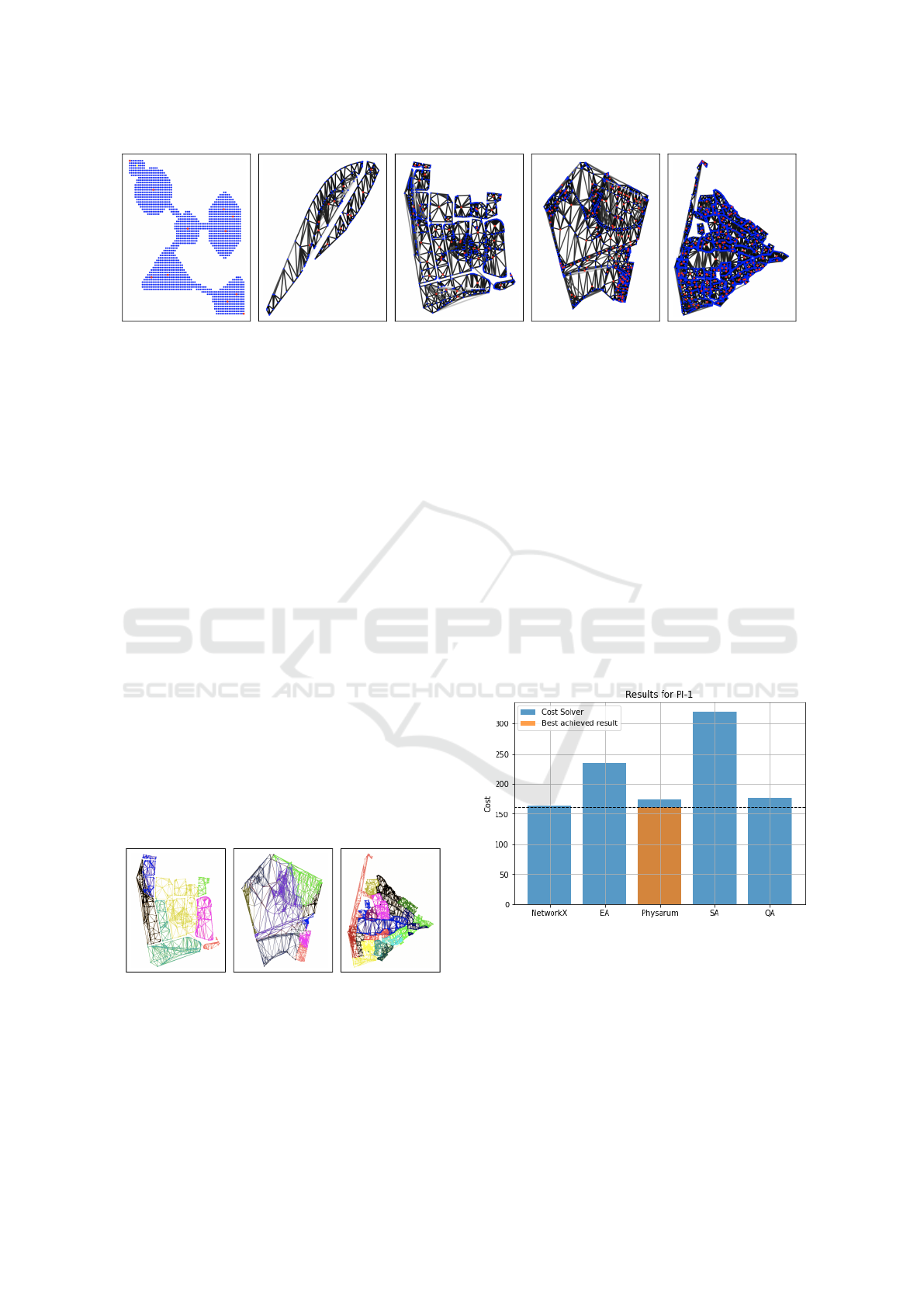
(a) PI-1(1560, 4294) (b) PI-2(158, 458) (c) PI-3(888, 2578) (d) PI-4(1463, 5268) (e) PI-5(3859, 11163)
Figure 3: Benchmark problem instances denoted PI-X(N, E) with varying numbers of nodes (N) and edges (E).
4.2 Partitioning
It is assumed that solvers produce more cost-efficient
solutions of large Steiner Trees if large input graphs
are partitioned into smaller subgraphs. Some well-
partitioned input graphs can be seen in Figure 4,
where different colors correspond to different sub-
graphs.
GM partitioning is well suited for smaller graphs
with a low degree of connectivity between clusters
(e.g. PI-1).
Voronoi-based partitioning produces well-
separated subgraphs for bigger graphs with a low
number of connections between subgraphs (see Fig-
ure 4a). Spectral Clustering produces good clusters
on all complexity levels. However, the predefined
number of clusters based on Voronoi or Eigengaps
seems to make a difference, especially for graphs
with a strong meshing (e.g. PI-5).
To summarize, GM partitioning works best for in-
put graphs with visible clusters and a low number
inter-cluster connections. If sparse graphs get larger,
using partitioning Voronoi-based partitioning should
produce better results. For dense graphs, Spectral
Clustering is the best choice.
(a) Voronoi (b) SC (EG) (c) SC (V)
Figure 4: Comparison of partitioning methods: Voronoi
(V), Spectral Clustering (with Eigen Gaps (EG) or
Voronoi).
4.3 Network Cost
Figure 5 shows the lowest achieved network cost for
each solver for PI-1 without partitioning or simpli-
fying (except for Quantum Annealing, where prior
simplifying is necessary due to hardware constraints).
For better comparison, the best overall result with en-
abled partitioning is also included. The NetworkX
solver outperforms all others. However, the Physarum
and Quantum Annealing solvers show slightly worse,
but competitive results. The best overall result was
achieved by a combination of Physarum and Greedy
Modularity partitioning. There, the baseline is outper-
formed by 1.22%. Interestingly, a partitioner or sim-
plifier combined with the NetworkX approach results
in increased cost.
Figure 5: Network costs for PI-1. The blue bars show the
best result achieved for each solver on the input graph with-
out partitioning or simplification (except QA). As a refer-
ence, the orange bar shows the best overall result. This was
achieved by a combination of Physarum and Greedy Mod-
ularity partitioning.
A similar correlation is visible for real-life prob-
lem instances. Figure 6 shows the results of each
solver. Again, Quantum Annealing is the only algo-
rithm with prior simplifying. NetworkX, Physarum
Solving Large Steiner Tree Problems in Graphs for Cost-efficient Fiber-To-The-Home Network Expansion
29

and Quantum Annealing return the most cost-efficient
solutions, outperforming the Evolutionary Algorithm
and Simulated Annealing. Please note that PI-5 could
only be solved by NetworkX and Physarum without
the help of partitioners or simplifiers.
Figure 6: Resulting costs for PI-2 to PI-5 for each solver.
Every possible combination of simplifier, parti-
tioner and solver was evaluated on each instance. Fig-
ure 7 shows the best overall result compared with the
NetworkX baseline. The number above each prob-
lem denotes the cost improvement in percent. Hence,
the baseline could be outperformed on PI-2 by 0.56%,
PI-3 by 1.57% and PI-4 by 0.32%. Except for PI-
2, these enhancements have been achieved with prior
partitioning.
Figure 7: Comparison of baseline and best achieved results.
The number above each problem denotes the cost improve-
ment in percent. A negative value corresponds to a cost
improvement.
Table 1 contains a more detailed overview of the
lowest achieved costs for each solver and problem in-
stance. Additionally, the combination of simplifier,
partitioner and solver which returned the best result
for each problem are highlighted. In summary, the
NetworkX baseline could be outperformed on 4 out of
5 problem instances. Physarum in combination with
prior partitioning is the overall most cost-efficient ap-
proach, where the choice of the partitioning scheme
depends on the initial graph. Furthermore, simplifica-
tion does not further reduce the lowest costs for any
of the evaluated problem instances.
Table 1: Network cost for different solvers: NetworkX
baseline, Evolutionary Algorithm (EA), Physarum, Simu-
lated Annealing, Quantum Annealing (QA). Other abbre-
viations: Growing Neural Gas (GNG), Spectral Clustering
(SC), Greedy Modularity (GM), Triangulation (Triangle).
Problem Approach Cost
PI-1
N = 1560
E = 4294
NetworkX 164.0
EA 235.0
Physarum (5 runs) 174.0
Simulated Annealing 320.0
QA (Leap) + GNG + SC
(Voronoi)
175.0
Physarum + GM 162.0
PI-2
N = 158
E = 458
NetworkX 0.006679
EA 0.062119
Physarum (5 runs) 0.006641
Simulated Annealing 0.042000
QA (qbsolv) + Triangle 0.007861
PI-3
N = 888
E = 2578
NetworkX 0.041419
EA 0.286315
Physarum (5 runs) 0.045759
Simulated Annealing 0.249000
QA (Leap) + GNG 0.042000
Physarum + SC 0.040768
PI-4
N = 1463
E = 5268
NetworkX 0.051680
EA 0.375550
EA + NetworkX 0.051514
Physarum (5 runs) 0.063590
Simulated Annealing 0.250000
QA (qbsolv) + GNG + SC
(Voronoi)
0.072522
PI-5
N = 3859
E =
11163
NetworkX 0.175814
EA -
Physarum (5 runs) 0.206857
Simulated Annealing -
QA (qbsolv) + GNG +
Voronoi
0.280829
4.4 Duration
Figure 8 shows the computation time for each solver
and problem instance. Quantum Annealing was ex-
cluded from this graph since prior simplifying was
needed and this would drastically affect computation
time. The NetworkX baseline is the fastest approach
throughout all instances with small increases for each
complexity level. The Evolutionary Algorithm and
Physarum mostly show similar results, still outper-
forming Simulated Annealing. However, Physarum
shows a large spike for PI-5, returning the result after
almost 233 minutes compared to 36 minutes for PI-4.
ICAART 2022 - 14th International Conference on Agents and Artificial Intelligence
30

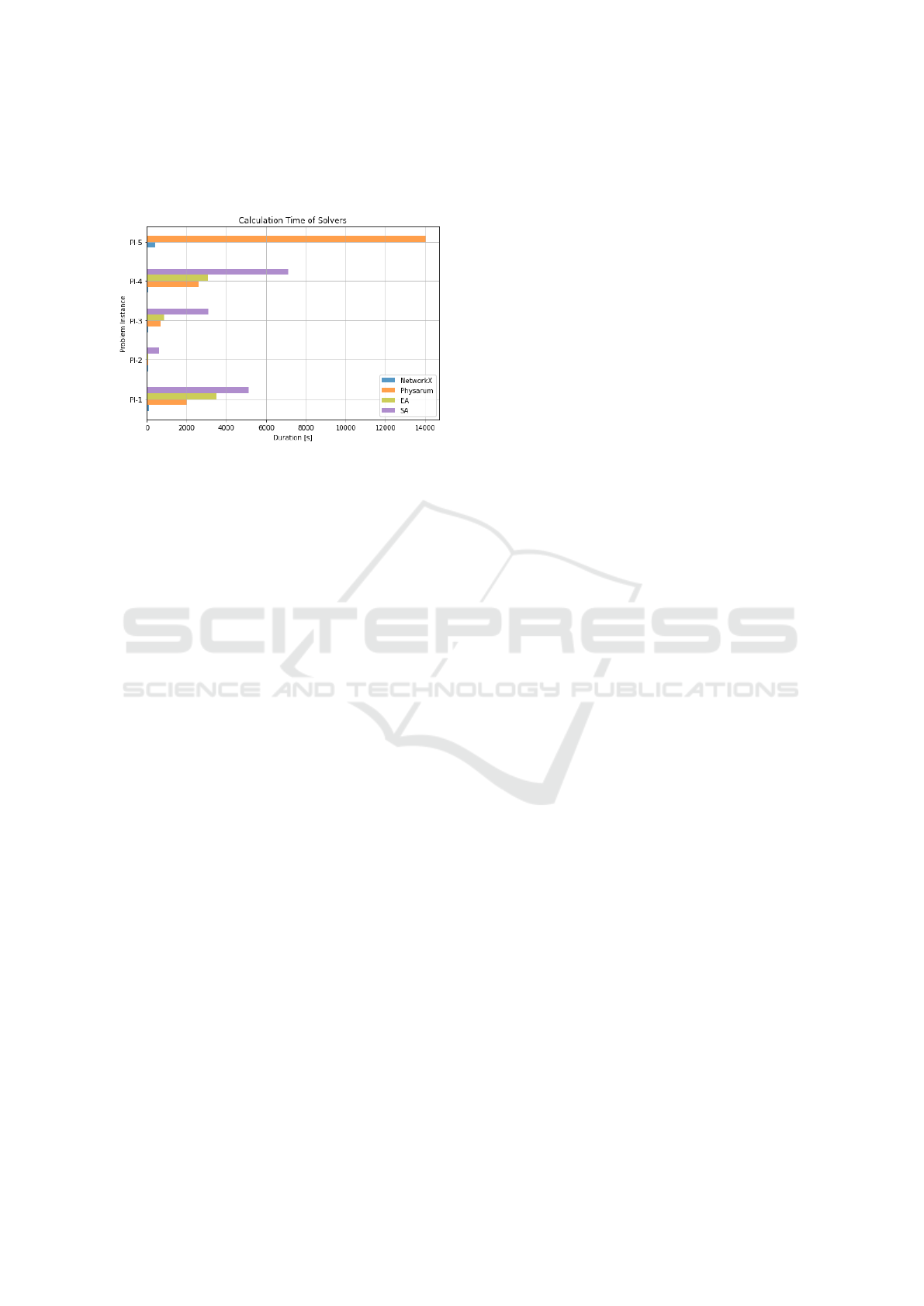
This effect could be reduced by partitioning but since
the baseline algorithm could not be outperformed on
this instance, no further experiments were conducted.
Figure 8: Computation times for all solvers and problem
instances in [s].
5 RELATED WORK
Even though Steiner Tree Problems have already been
studied for decades (Duin and Voß, 1994; Promel and
Steger, 2002), it has been revisited repeatedly with a
high variety of approaches.
For example, Rosenberg et al. (Rosenberg et al.,
2021) developed and successfully applied Evolution-
ary Algorithms to Euclidean STPs with soft obsta-
cles and up to 1000 nodes. Despite needing a rela-
tively long time to converge, the approach was able
to outperform an iterative approach in terms of cost-
efficiency and showed promising results.
In (Siebert et al., 2020) a technique based on
Dynamic Programming and neighborhood structure
characterization was proposed, which also uses Simu-
lated Annealing. Recently, work on using gate-model
Quantum Computers for solving the STP has been
published (Miyamoto et al., 2020). In their pub-
lication, Miyamoto et al. have devised a hybrid-
quantum algorithm based on Grover’s search algo-
rithm (Grover, 1996) that has a time complexity better
than classical state-of-the-art algorithms. However,
no experimental results are available and there exist
no statements on necessary error correction strategies
or on its applicability on Noisy Intermediate-Scale
Quantum Computers (NISQ).
6 CONCLUSION
In this work, a wide range of state-of-the-art algo-
rithms for simplifying, partitioning and solving large
STPs was introduced and discussed. The proposed
algorithms were evaluated on multiple real-life prob-
lem instances and compared against a widely used
baseline algorithm which could be outperformed on
4 out of 5 instances. Even though good partitioning
was key for achieving high network cost-efficiency, it
is assumed that the partitioning and merging process
affects result optimality negatively. Further work to-
wards optimal partitioning of Steiner Trees might lead
to better results. Also, input graph simplification did
not lead to a further decrease in network costs.
Although computational time is comparatively
long for Physarum, it is reasonable to leverage
this approach since it outperformed the baseline by
about 1% on 3 out of 5 instances, which, due to
high excavation costs, makes a significant contri-
bution to cost savings when expanding FTTH net-
works. Hence, longer runtime is mostly compen-
sated by cost-efficiency, especially when approximat-
ing district-sized FTTH networks. Larger networks
with a high degree of connectivity (PI-4 and PI-5)
could not be outperformed by Physarum. However,
the results on these instances could potentially be im-
proved through better partitioning.
While Quantum Annealing hardware is not yet us-
able to solve STP instances with sizes relevant to our
application domain, experiments have shown that run-
ning Quantum Annealing algorithms on simulators or
hybrid software already returns decent results, espe-
cially for smaller problem instances. This indicates
that performing experiments on future Quantum An-
nealers with more physical qubits might still be of in-
terest. There seems to be a trend for the number of
qubits in Quantum Annealers to double every two to
three years (McGeoch and Farr
´
e, 2020). In combi-
nation with a potentially more efficient QUBO for-
mulation (Fowler, 2017), it should thus be possible
to solve STP instances for FTTH networks of rele-
vant size within the next decade. With the help of
sophisticated partitioners and simplifiers, this should
be achievable even sooner.
ACKNOWLEDGEMENTS
The authors would like to thank Deutsche Telekom
Laboratories (T-Labs) for funding this work.
REFERENCES
Adamatzky, A. (2014). Route 20, autobahn 7, and slime
mold: Approximating the longest roads in usa and ger-
Solving Large Steiner Tree Problems in Graphs for Cost-efficient Fiber-To-The-Home Network Expansion
31

many with slime mold on 3-d terrains. IEEE Transac-
tions on Cybernetics, 44(1):126–136.
Adamatzky, A. and Prokopenko, M. (2012). Slime mould
evaluation of australian motorways. International
Journal of Parallel, Emergent and Distributed Sys-
tems, 27(4):275–295.
Clauset, A., Newman, M. E. J., and Moore, C. (2004). Find-
ing community structure in very large networks. Phys-
ical Review E, 70(6).
Duin, C. and Voß, S. (1994). Steiner tree heuristics — a sur-
vey. In Operations Research Proceedings 1993, pages
485–496, Berlin, Heidelberg. Springer Berlin Heidel-
berg.
Fowler, A. (2017). Improved qubo formulations for d-wave
quantum computing. Master’s thesis, University of
Auckland, Auckland, New Zealand.
Fritzke, B. (1994). A growing neural gas network learns
topologies. Advances in neural information process-
ing systems, 7:625–632.
Grover, L. K. (1996). A fast quantum mechanical algorithm
for database search. In Proceedings of the Twenty-
Eighth Annual ACM Symposium on Theory of Com-
puting, STOC ’96, page 212–219, New York, NY,
USA. Association for Computing Machinery.
Gupta, A. and K
¨
onemann, J. (2011). Approximation algo-
rithms for network design: A survey. Surveys in Op-
erations Research and Management Science, 16(1):3–
20.
Hagberg, A. A., Schult, D. A., and Swart, P. J. (2008). Ex-
ploring network structure, dynamics, and function us-
ing networkx. In Varoquaux, G., Vaught, T., and Mill-
man, J., editors, Proceedings of the 7th Python in Sci-
ence Conference, pages 11 – 15, Pasadena, CA USA.
Hwang, F. K. and Richards, D. S. (1992). Steiner tree prob-
lems. Networks, 22(1):55–89.
Kapsalis, A., Raywad-Smith, V., and Smith, G. D. (1993a).
Solving the graphical steiner tree problem using ge-
netic algorithms. Journal of the Operational Research
Society, 44(4):397–406.
Kapsalis, A., Rayward-Smith, V. J., and Smith, G. D.
(1993b). Solving the graphical steiner tree problem
using genetic algorithms. The Journal of the Opera-
tional Research Society, 44(4):397–406.
Lehner, B., Umlauf, G., and Hamann, B. (2008). Video
compression using data-dependent triangulations.
Leitner, M., Ljubi
´
c, I., Luipersbeck, M., and Resch, M.
(2014). A partition-based heuristic for the steiner tree
problem in large graphs. In International Workshop
on Hybrid Metaheuristics, pages 56–70. Springer.
Liu, L., Song, Y., Zhang, H., Ma, H., and Vasilakos, A.
(2015). Physarum optimization: A biology-inspired
algorithm for the steiner tree problem in networks.
IEEE Transactions on Computers, 64:819–832.
Lucas, A. (2014). Ising formulations of many np problems.
Frontiers in Physics, 2:5.
Madras, N. N. (2002). Lectures on monte carlo methods,
volume 16. American Mathematical Soc.
McGeoch, C. and Farr
´
e, P. (2020). The d-wave advantage
system: An overview. Technical Report 14-1049A-A,
D-Wave Systems Inc., Burnaby, BC, Canada.
Metropolis, N., Rosenbluth, A. W., Rosenbluth, M. N.,
Teller, A. H., and Teller, E. (1953). Equation of state
calculations by fast computing machines. The journal
of chemical physics, 21(6):1087–1092.
Miyamoto, M., Iwamura, M., Kise, K., and Gall, F. L.
(2020). Quantum speedup for the minimum steiner
tree problem. In Kim, D., Uma, R. N., Cai, Z., and
Lee, D. H., editors, Computing and Combinatorics,
pages 234–245, Cham. Springer International Pub-
lishing.
Promel, H. and Steger, A. (2002). The steiner tree problem:
A tour through graphs algorithms and complexity.
Pr
¨
omel, H. J. and Steger, A. (2012). The Steiner tree prob-
lem: a tour through graphs, algorithms, and complex-
ity. Springer Science & Business Media.
Rosenberg, M., French, T., Reynolds, M., and While, L.
(2021). A genetic algorithm approach for the eu-
clidean steiner tree problem with soft obstacles. In
Proceedings of the Genetic and Evolutionary Compu-
tation Conference, GECCO ’21, page 618–626, New
York, NY, USA. Association for Computing Machin-
ery.
Shi, J. and Malik, J. (2000). Normalized cuts and image
segmentation. IEEE Transactions on Pattern Analysis
and Machine Intelligence, 22(8):888–905.
Siebert, M., Ahmed, S., and Nemhauser, G. (2020). A sim-
ulated annealing algorithm for the directed steiner tree
problem.
Sun, Y. (2019). Solving the steiner tree problem in graphs
using physarum-inspired algorithms.
Venegas-Andraca, S. E., Cruz-Santos, W., McGeoch, C. C.,
and Lanzagorta, M. (2018). A cross-disciplinary in-
troduction to quantum annealing-based algorithms.
Contemporary Physics, 59(2):174–197.
Zelnik-Manor, L. and Perona, P. (2004). Self-tuning spec-
tral clustering. In Advances in Neural Information
Processing Systems 17, pages 1601–1608. MIT Press.
ICAART 2022 - 14th International Conference on Agents and Artificial Intelligence
32