
A New Method of Dimensionality Reduction for Large Time Series
Applied to Accelerometer Wristbands’ Signals
Alihu
´
en Garc
´
ıa-Pavioni and Beatriz L
´
opez
Exit Group, University of Girona, Catalonia, Spain
Keywords:
Accelerometers Wristbands, High-dimensional Time Series, Time Series Classification, Dimensionality
Reduction, Feature Extraction, Behavior Recognition, Signal State Changes.
Abstract:
Feature extraction for high-dimensional time series has become a topic of great importance in recent years. In
the medical field, the information needed to predict emotions, stress, epileptic seizures, heart attacks, Parkin-
son, fall detection in the elderly, and other diseases, can be provided by body sensors in the form of time series
signals. The commercial usage of wearable accelerometers has also made the study of time series activity
recognition gain much attention. Thus, as the time series provided by the accelerometers could be really long,
consuming a lot of storage data and also hamming the machine learning classifier accuracy results, it is im-
portant to identify which features are relevant in this particular context, so the data stored can consume the
least amount of memory possible in the device, while at the same time the activity classification performance
would be satisfactory. This work intends to provide a way for these devices to save the relevant information
needed for the machine learning activity classification, by defining a new feature extraction method. The
method proposed in this work, called State Changes Representation for Time Series (SCRTS), relies on the
relevant data associated with the “state changes” in the time series. These changes are identified according
to the conditional probabilities of passing from one state to another during the time, and the “relevance” of
each state. We show the results of this method with an experiment based on accelerometers data recorded by
the ©ActiGraph wGT3X-BT wristband to recognize sedentary behavior. After applying this method, it was
achieved to reduce time series frames of dimension 360, to vectors of dimension 12; while their classification
accuracy was 84%.
1 INTRODUCTION
The study of time series feature extraction and clas-
sification has become of great importance in the last
years. A time series is a succession of values mea-
sured in time and arranged chronologically. Its feature
extraction and classification has many applications in
healthcare, medicine, veterinary, biology, economy,
and engineering, among others.
In the medical field particularly, the development
and popularization of easily accessible wearable de-
vices outputting time series has led to increased the
attention considerably in this topic. In this sense, the
development of time series classification techniques
has become very relevant. The usage of wearable
devices with machine learning algorithms to clas-
sify time series can be applied to predict emotions,
stress, epileptic seizures, heart attacks (Montesinos
et al., 2019; Shoeb and Guttag, 2010; Wang et al.,
2014; Ravish et al., 2014), and other diseases such
as Parkinson (Rastegari et al., 2019), or fall detection
in the elderly (Sanchez and Mu
˜
noz, 2019; Li et al.,
2017; Howcroft et al., 2017).
The commercial usage of wearable accelerome-
ters has also made the study of activity recognition
gain much attention. For example, with an appro-
priate machine learning algorithm, a wearable ac-
celerometer can be used for monitoring a person daily
life activities, to give a warning in case that an el-
derly or disabled person has fallen down, or to have
a record of the weekly physical activities made by
some user, among many other usages. Thus, as the
time series provided by the accelerometers could be
really long, therefore consuming a lot of storage data
and also hamming the machine learning classifier ac-
curacy results, it is important to identify which fea-
tures are relevant in this particular context, so the data
stored can consume the least amount of memory pos-
sible in the device, while at the same time the activity
classification performance would be satisfactory.
García-Pavioni, A. and López, B.
A New Method of Dimensionality Reduction for Large Time Series Applied to Accelerometer Wristbands’ Signals.
DOI: 10.5220/0010672800003123
In Proceedings of the 15th International Joint Conference on Biomedical Engineering Systems and Technologies (BIOSTEC 2022) - Volume 4: BIOSIGNALS, pages 103-110
ISBN: 978-989-758-552-4; ISSN: 2184-4305
Copyright
c
2022 by SCITEPRESS – Science and Technology Publications, Lda. All rights reserved
103

This work intends to provide a way for these de-
vices to save the relevant information, using little
storage memory, by defining a new feature extrac-
tion method, called State Changes Representation for
Time Series (SCRTS). Different to other methods in
the literature, the SCRTS relies on the relevant data
associated with the time series “state changes”. These
changes are identified according to the conditional
probabilities of passing from one state to another dur-
ing the time and the “relevance” of each state, pro-
viding the information needed to represent or charac-
terize an accelerometer time series in the context of
activity recognition.
To test our method we conduct an activity classi-
fication experiment with people in our lab, trying to
determine when they were in the office or when they
were not, based on their behaviors described through
the time series provided by the usage of ©ActiGraph
wGT3X-BT wristbands accelerometers. Eight PhD’s
and master students working at the same office in the
University of Girona, wore these wristbands on their
skillfully wrist for approximately 9 days, which were
programmed to record a measure every ten seconds.
A total of 1582 hours of time series data was collected
from these devices. Then we applied the SCRTS al-
gorithm to select the relevant data, that in the case of
one-hour frames it was achieved to reduce time series
frames of dimension 360 to vectors of dimension 12;
and after that, we implemented an artificial neural net-
work to do the classification, achieving an accuracy of
84%.
2 LITERATURE SURVEY
Time series feature extraction (TSFE) is essential for
machine learning effectiveness in time series classifi-
cation problems, on the one hand because it reduces
the dimension of the feature space, and on the other,
because it has a significant impact on the final results,
since it transforms the input data in vectors easier to
interpret by the machine learning classification algo-
rithm.
There exist many different TSFE methods. The
Fourier Transform (Bracewell and Bracewell, 1986)
and the Wavelet Transform (Shensa, 1992), which are
very classical, could be very useful applied to time se-
ries composed mostly of periodic waves, like it hap-
pens with the EEG signals, or other signals related
to the light, the electricity, the image, or the sound,
among others. But when it comes to analyse time se-
ries that does not present a periodic behavior, such as
the data extracted from an accelerometer, this meth-
ods may not work well.
There exist other classical statistical methods for
feature extraction like the Singular Value Decom-
position (SVD)(Cadzow et al., 1983), the Principal
Component Analysis (PCA) (Wold et al., 1987), or
the Linear Discriminant Analysis (LDA) (Izenman,
2013). These methods use Linear Algebra tools for
reducing the information of the input matrix. They
work well for static data, but when it comes to time
series, it may present some problems. We are inter-
ested in exploring the scope of selecting features that
contain information about the changes, and we con-
sider that this information is in its conditional proba-
bilities related to the states and the relevance of each
state.
In (Kate, 2016) distance-based methods like dy-
namic time warping (DTW) with feature-based meth-
ods like SAX are combined using DTW to create new
features which are then given to a standard machine
learning method. In (Zhou and Chan, 2015) a method
called Multivariate Time Series Classifier (MTSC) is
proposed, using conditional probabilities to create a
measure that allows to discover some intra and inter-
temporal patterns. In this work we make use of the
conditional probabilities as well, but instead of seek-
ing for these intra and inter-temporal patterns, we
seek for other features that could give a description
of how much the signal has changed inside of each
period, relating these changes with the activity made
by the wristband’s user.
In the particular case of activity classification us-
ing accelerometer data, in (Pavey et al., 2017) a ran-
dom forest activity classifier to recognize four activ-
ity classes using an accelerometer wristband is devel-
oped. In (Ellis et al., 2014) a classification of four dif-
ferent activities using frequency and time domain fea-
tures in accelerometers is made, and then in a follow-
up work (Ellis et al., 2016), a technique using random
forest and a hidden Markov model for classifying four
activities is performed. In (Sasaki et al., 2016) time
and frequency domain features were extracted from
the accelerometers signals to be classified with ran-
dom forest into five activity classes. In (Mannini and
Intille, 2018) an approach for personalizing classifi-
cation rules to a single person is proposed. In (Lee
and Kwan, 2018) an approach to classifying physical
activity using Fast Fourier Transform applied to pub-
lished smartphone accelerometer data with random
forest and gradient boosting is presented. In (Ahmadi
et al., 2020) different machine learning algorithms to
predict children’s physical activity are developed and
evaluated. In (Mohamed et al., 2018) the multi-label
classification technique with the Label Combination
using Fourier analysis for the feature extraction is
proposed, investigating the role of sensor placements
BIOSIGNALS 2022 - 15th International Conference on Bio-inspired Systems and Signal Processing
104

for recognizing various types of physical activities.
In (Wang et al., 2016) the ensemble empirical mode
decomposition (EEMD)-based features is introduced,
and a game theory-based feature selection method is
proposed to evaluate the features. In (Zubair et al.,
2016) activity classification is performed using ran-
dom forest and decision tree in connection with Ad-
aBoost. In (Tian et al., 2020) wavelet energy spectrum
features and a novel feature selection method are in-
troduced and an ensemble-based filter feature selec-
tion (EFFS) approach to optimize the feature set is
proposed, using for the final classification k-nearest
neighbour and support vector machine.
Although many of the presented techniques for ac-
tivity classification have shown to work well, none
of them has explored the scope of using the condi-
tional probabilities between the states together with a
measure of the relevance of these states, as features
to be used in the machine learning classifier. There-
fore, the purpose of this work is to study the scope
of using this features for activity classification. The
algorithm proposed for this, the SCRTS, discretizes
the range of possible time series’ values into differ-
ent “states”, and extracts the information of how these
states “change” (that is to say, which values take the
conditional probabilities), and how much importance,
or “weight”, these states had in the frames that we
want to classify.
3 METHODOLOGY
Fig. 1 shows the different steps of the methodology,
detailed in this section.
3.1 Data Collection
A time series is a succession of values measured in
time and arranged chronologically. As we made use
of accelerometers to obtain the data, we refer to the
values of the time series as vector magnitudes, and
we refer to a vector magnitude value as V M, which is
defined as
V M =
q
(a
x
)
2
+ (a
y
)
2
+ (a
z
)
2
, (1)
were a
x
, a
y
, a
z
are the accelerations measured by the
wristband in axis x, y, z respectively. We refer as τ to
the time frequency with which these vectors magni-
tudes are displayed by the device.
3.2 Division Into Frames
Every time signal was divided in frames of T min-
utes. So far, every frame is represented by a vector
of dimension d equal to the number of samples in it.
Then, we denote each frame as a vector F such that:
F = (V M
i
)
i≤d
. (2)
Therefore, in the experiment presented in this
work, as every value is given every ten seconds (i.e.,
τ = 10 seconds), if for example we choose our T = 60
minutes, we have that each frame has a dimension of
d = 360.
3.3 Discretization
There are many different methods for time series tem-
poral discretization (Moskovitch and Shahar, 2015;
Azulay et al., 2007), which involves to obtain a se-
quence of states from a numerical time series. These
states are domain dependent. This means that, if we
look at the time series, with axis y being the vector
magnitude values and axis x the time, then the y axis
is divided by several cut points into n intervals, each
of them representing a state.
Formally, given a set of cut points
CP = {cp
0
, cp
1
, . . . , cp
n
}, (3)
we can generate a set Σ of n states, each state S
i
∈
Σ representing an interval of the vector magnitudes
values made by the cut points, as follows:
S
1
= [cp
0
, cp
1
),
S
2
= [cp
1
, cp
2
), (4)
.
.
.
S
n
= [cp
n−1
, cp
n
],
where cp
0
and cp
n
are the time series’ minimum and
maximum values respectively.
We say that a vector magnitude VM is of state S
i
,
when V M ∈ S
i
, that is to say, when cp
i−1
≤V M ≤ cp
i
.
Consistently, given a set of states Σ, we can represent
each frame F by a sequence of states
S(F) = {S
1
, S
2
, . . . , S
d
}, (5)
where S
t
∈ Σ, and the supra-index t indicates the
chronological position of the state in the frame.
3.4 Conditional Probabilities
Given a frame F of our time-signal represented by
S(F) = {S
1
, S
2
, . . . , S
d
}, the conditional probability of
getting state S
t+1
= b after being in state S
t
= a, with
a, b ∈ Σ, is defined as
Prob(S
t+1
= b | S
t
= a) =
Frec(a, b)
Frec(a)
, (6)
A New Method of Dimensionality Reduction for Large Time Series Applied to Accelerometer Wristbands’ Signals
105
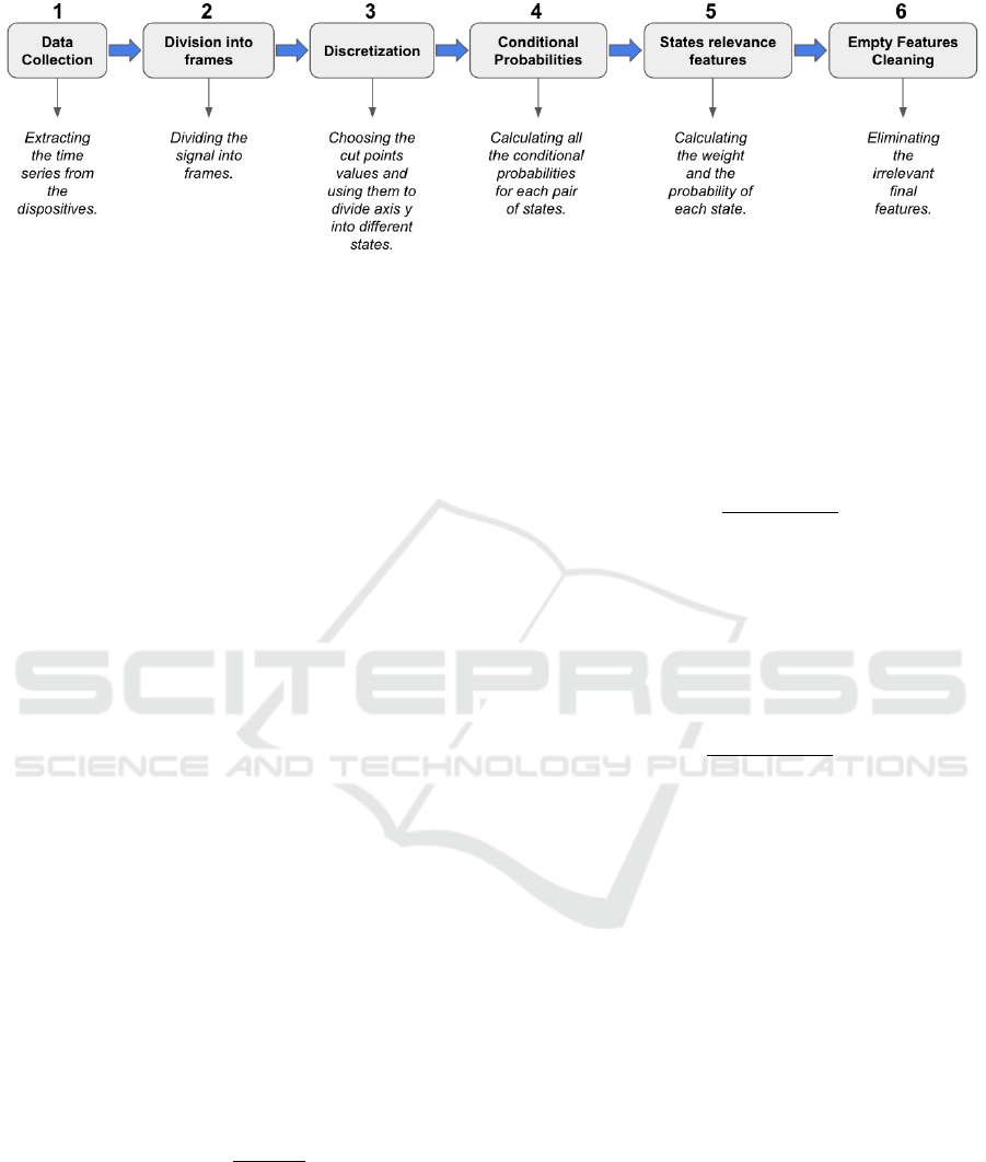
Figure 1: SCRTS steps.
such that 1 ≤ t ≤ d − 1, being Frec(a, b) the num-
ber of times that a is followed by b in S(F) =
{S
1
, S
2
, . . . , S
d
}, and Frec(a) the number of times that
a appears in {S
1
, S
2
, . . . , S
d−1
}.
Therefore, we calculate every conditional proba-
bility for each frame, which gives us a total of n
2
features per frame in each case. Thus, we use these
features for making a new vector for representing the
information contained in frame F. We call C(F) to
refer to the vector of all the conditional probabilities
of F.
C(F) reflect the “jumps” from one state to another,
giving a description of the changes or the “stays”,
showing which jumps were more common in F, and
which states stay longer without changing.
3.5 States Relevance Features
But C(F) does not give any information about the
“relevance” of each state in the time series, or about
which of them have appeared a greater number of
times. Though, if we want to create a vector that
contains most of the state’s changes relevant features,
then we should probably include relevant data regard-
ing to the states appearance in the frame. To that end,
we make usage of two features: the state probability,
and the state weight.
3.5.1 State Probability
For each S
i
∈ Σ, the probability of state S
i
to come out
in frame F is:
P(S
i
) =
Frec(S
i
)
d
. (7)
Therefore, we refer to the set of all the state probabil-
ities of a frame F as P(F), that is to say
P(F) = {P(S
1
), P(S
2
), . . . , P(S
n
)}. (8)
3.5.2 State Weight
As we already said in (4), for every state S
i
∈ Σ, we
have a cp
i−1
and a cp
i
indicating the rang for a vector
magnitude V M to be labelled as state S
i
. Then, we
define the midpoint of each state S
i
∈ Σ as
mid
i
=
(cp
i
+ cp
i−1
)
2
. (9)
The distance from the midpoint to the top of state S
i
is
dis
i
= |mid
i
− cp
i
|
= |mid
i
− cp
i−1
|
. (10)
Now, for every V M belonging to a state S
i
we can
define the normalized inverted distance of V M to it’s
respective midpoint mid
i
of S
i
, as
NID
i
(V M) =
−|mid
i
−V M|
dis
i
+ 1. (11)
For the reader familiar with statistics, the normalized
inverted distance is similar to the z-score function
(Kreyszig, 2009). The difference is that the normal-
ized inverted distance is like making 1 − z-score, but
instead of dividing by the standard deviation, in the
normalized inverted distance we divide by the dis-
tance from the midpoint to the top of its respective
state interval.
The importance of the NID
i
is that it gives and
idea of how “weighted” V M is for state S
i
. If V M lies
in the midpoint of the state S
i
, the NID
i
is 1, which
is the maximum value possible; and the further it lies
from the midpoint, the lower the NID
i
is, being 0 at
the lower and upper values of S
i
, that is to say,
NID
i
(mid
i
) = 1; (12)
NID
i
(cp
i
) = NID
i
(cp
i−1
) = 0. (13)
Thus, if we sum all the NID
i
’s of all the vector
magnitudes laying in a state S
i
∈ Σ for a frame F, and
we normalize the result, then we have a notion of how
much “weight” or relevance has S
i
in F. Let’s say
that Q(S
i
) = {V M
1
, V M
2
, . . . , V M
q
} is the set of all
BIOSIGNALS 2022 - 15th International Conference on Bio-inspired Systems and Signal Processing
106

the vector magnitudes of the frame F laying in state
S
i
, then, we define the weight of state S
i
in F as
W (S
i
) =
∑
q
j=1
NID
i
(V M
j
)
d
, if Q(S
i
) 6=
/
0;
0, if Q(S
i
) =
/
0;
(14)
where d is the amount of vector magnitudes in F =
(V M
j
)
j≤d
. We refer to all the state weights of a frame
F as W (F), that is to say
W (F) = {W (S
1
), W (S
2
), . . . , W (S
n
)}, (15)
with n being the number of states in Σ (as we already
said in (4)).
Though, the dimension of these vectors depend on
the number of states. Let’s call dim(V ) to the function
that returns the dimension of a vector V , then
dim(C(F)) = n
2
; (16)
dim(P(F)) = dim(W (F)) = n. (17)
Finally, we call as the representation vector R(F)
to the vector containing the features selected to repre-
sent F according to our method. These features are:
C(F), P(F) and W (F). Though, the dimension of
R(F) is
dim(R(F)) = n
2
+ 2n. (18)
3.6 Empty Features Cleaning
The SCRTS is, as the name says it, a method for rep-
resenting time series. This is to say that our goal is to
extract all the relevant data of all the frames involved
so they can be used as a matrix for a machine learning
algorithm. This matrix has every R(F) of each frame
F as rows. So each column of the matrix represents
a different feature of the frames. Therefore, there is a
column for each conditional probability, one for every
weight, etc. If one of these columns has more than a
75% of zeros means that the features of the column
are not relevant for representing the time series and it
could bring some noise for the machine learning per-
formance, then we delete it. This process will prob-
ably reduce the dimension of the training-test matrix
even more. As a result, the representation vector of
each frame will probably reduce its dimensionality.
4 EXPERIMENTAL SETUP
To test our method, we conduct an experiment with
people in our lab, trying to determine when they were
in the office or when they were not, based on their
behaviors described through the time series provided
by the usage of ©ActiGraph wGT3X-BT wristbands
accelerometers.
Eight PhD’s and master students working at the
same office in the University of Girona, wore these
wristbands on their skillfully wrist for approximately
9 days, which were programmed to record a measure
every ten seconds (i.e., τ = 10 seconds). A total of
1582 hours of time series data was collected from
these devices.
The subjects were asked to take note of their office
check-in and check-out times for each day using the
wristband. Next, when dividing the signal into frames
of T minutes duration, each frame was labeled with 1
if the subject was more than half of that time at the
office, or with 0 otherwise.
We chose Freedson Adult 1998 cut points pro-
vided by ActiLife (Freedson et al., 1998) for the dis-
cretization, which give us a total of 5 states (i.e.,
n = 5)
1
.
4.1 Classification
The classification of frames between classes {0,1}
was made using sequential Artificial Neural Networks
(ANN)
2
. It had 8 hidden layers of 12 nodes and the
Relu activation function in each layer. The output
layer was a dense layer with 2 nodes and the Sigmoid
activation function. The optimizer was Adam with a
learning rate of 0.001 units; the loss function was the
binary crossentropy and the number of epochs was 40.
No overlapping was applied in the frames divi-
sion. All the data frames were randomly shuffle to-
gether and split into the training set (75%) and the test
set (25%). We applied random oversampling (Ling
and Li, 1998) to level the quantity of frames in the
training set labeled with 1 with the ones labeled with
0. The accuracy, the true positive rate (TPR) and the
true negative rate (TNR), were calculated using the
test set. This procedure was executed 20 times, and
the final results were calculated as the average of the
results obtained in each of the 20 performances.
5 RESULTS
We applied the SCRTS to the data of all the wrist-
bands together. The results achieved have been com-
pared with the ones obtained from the same physio-
1
We also tried with the cut points provided by Actil-
ife called Freedson Adult VM3 2011, Trost Toddler 2011,
and Troiano 2008, but Freedson Adult 1998 were the ones
which gave us better results in this experiment.
2
We also tested other architectures, as LSTM and SVM,
with similar results.
A New Method of Dimensionality Reduction for Large Time Series Applied to Accelerometer Wristbands’ Signals
107

logical signals without any feature extraction method,
that is, using the raw data directly. Different frame
lengths were explored: T = 15, T = 30 and T = 60
minutes. The results with the final dimension of the
vectors representing the frames for the classification
(Dim.), the accuracy (Acc.), the true positive rate
(TPR) and the true negative rate (TNR) are provided
in Table 1.
The first aspect to notice looking at this table is
that working with the SCRTS gave much better results
than working with the raw data, specially for long pe-
riods. One other thing is that the dimensionality re-
duction with the SCRTS is considerable compared to
the raw data. In the best case (T = 60), the dimension
of each frame was reduced from 360 to 12 with the
SCRTS, while the accuracy was 84%, the TPR 81%,
and the TNR 84%.
In Table 2 it is shown the results obtained after
applying the SCRTS to the data of each wristband (W)
individually, with T = 60 minutes. It could be seen
that the SCRTS also works well in the classification
of the time series individually.
The different works in the literature on activity
classification using accelerometers, show that the ac-
curacy varies considerably depending on the area of
the body where the devices were worn, as well as the
activity to be classified. In (Pavey et al., 2017) a ran-
dom forest activity classifier for recognize four activ-
ity classes (sedentary, stationary plus, walking, and
running) using an accelerometer wristband was devel-
oped, having an accuracy of 80.1%, 95.7%, 91.7%,
and 93.7%, respectively. In (Ellis et al., 2014) a clas-
sification of four activities (household duties, stair
climbing, walking, and running) using frequency and
time domain features was made, wearing the devices
on the hip and later on the wrist, having an overall ac-
curacy of 92.7% and 87.5%, respectively. In a follow-
up work (Ellis et al., 2016), a technique using random
forest and a hidden Markov model for classifying four
activities (sitting, standing, walking/running, and rid-
ing in a vehicle) was performed, using again the de-
vices on the hip and then on the wrist, obtained an av-
erage of 89.4% and 84.6% balanced accuracy over the
four activities, respectively. In (Sasaki et al., 2016)
time and frequency domain features were extracted
from the accelerometers signals used on the hip, wrist,
and ankle, to be classified with random forest into
five activity classes (sedentary, standing, household
chores, locomotion, and recreational activities), hav-
ing an accuracy of 87%, 84%, and 89% for the hip,
wrist, and ankle models, respectively. Then, look-
ing at the accuracy of these works performing activity
classification using wearable accelerometers (in the
hip, the wrist, or the ankle) in general, it can be seen
that the accuracy of the SCRTS algorithm applied
to the experiment explained in this work, is as good
as the ones obtained in these other works, although
some are slightly better. But looking specifically at
the ones using accelerometers wristbands for classi-
fying sedentary activities, it can be concluded that the
accuracy is in the same level, and in addition, a sig-
nificant dimensionality reduction was achieved, ex-
ploring also the usage of conditional probabilities be-
tween states, and what we defined as “state weights”,
as the features used in the machine learning classifier.
5.1 Discussion
The SCRTS algorithm has shown to have a good per-
formance in sedentary behaviors recognition using ac-
celerometers wristbands, as well as reducing signifi-
cantly the dimension of the frames. Even though, it
can probably be further improved in future works.
The SCRTS is an algorithm that combines a time
series discretization together with the computation
of its conditional probabilities and weights to repre-
sent the features to use in the machine learning al-
gorithm. Different results in the accuracy could be
obtained changing the discretization or the classifica-
tion algorithm. In this work we tried four different
cut points provided by Actilife, showing only the best
results with the cut points that suited better. We also
tried with Long short-term memory (LSTM) classifi-
cation algorithm and Support Vector Machine (SVM),
obtaining no better results than applying the ANN
architecture. This means that another discretization
techniques could be applied (Moskovitch and Shahar,
2015; Azulay et al., 2007), as well as another ma-
chine learning classification algorithms or architec-
tures, seeking to improve the accuracy.
Another consideration to take into account is that
when the participants were at the office, they went to
lunch, to the bathroom or did other activities besides
being working at their desks, wearing the wristbands
at all times. These activities are also in the period
labeled as they were at their desks, so it could bring
some noise to the experiment. If these particular pe-
riods were discarded (which is not possible with the
data we collected), the accuracy could probably be
improved.
Also, it should be noted that the particular time
we all had to live facing the pandemic of COVID-19,
put some limitations to this work as well. The experi-
ment was performed a few weeks before the confine-
ment was enacted in Spain, which generated too many
complications to get more data later on. We have been
able to get 8 persons to wear the accelerometers wrist-
bands for around 9 days. Although it may be seen as
BIOSIGNALS 2022 - 15th International Conference on Bio-inspired Systems and Signal Processing
108

Table 1: Results comparison using the SCRTS and the raw data.
T (min.) Dim. Acc. (%) TPR (%) TNR (%)
15 8 79 83 78
SCRTS 30 8 81 82 81
60 12 84 81 85
Raw 15 90 81 42 86
Data 30 180 80 42 86
60 360 16 9 97
Table 2: Results of SCRTS applied to each wristband individually.
W1 W2 W3 W4 W5 W6 W7 W8
Acc. (%) 84 77 84 84 89 83 89 78
TPR (%) 56 91 81 96 98 94 67 89
TNR (%) 86 74 84 82 87 80 96 77
not enough data since 8 participants is not much, it
is not the number of participants what really matters
for this experiment, but the number of long duration
frames acquired for the classification. The time series
collected represent a total of 1582 one-hour frames,
which we consider good enough to show a first scope
of the SCRTS algorithm. However, only two classi-
fication activities were performed by the participants.
Therefore, we are looking forward to try this algo-
rithm with some other data sets collected in a different
context.
6 CONCLUSIONS AND FUTURE
WORK
In this work we proposed a new method for dimen-
sionality reduction, the SCRTS, based on representing
how the signal information changes according to dif-
ferent states. In particular, state changes are modeled
with conditional probabilities, state probabilities and
state weights, which are used as features for the ma-
chine learning classification. This method has been
shown to work very well in a long time series clas-
sification problem. The classification for 60 minutes
frames gave an accuracy of 84%, a TPR of 81%, and a
TNR of 85%, while showing a lot of effectiveness for
storage, since it reduced the original data of dimen-
sion 360, to a vector of dimension 12.
This experiment was done with accelerometers
wristbands, which return one-channel time series per
user. In futures works we will try this technique with
the data collected by other wearable devices measur-
ing other body features, such as the electrocardio-
gram, the respiration, the skin temperature, the blood
volume pulse or the electrodermal activity. These
wearable devices return multi-channel time series for
each user, which add some complexity to our tech-
nique, so it will require some new treatments.
ACKNOWLEDGEMENTS
This work was carry out with the support of the Gen-
eralitat de Catalunya 2017 SGR 1551, and funded by
the Grants for the recruitment of new research staff
(FI), provided by the Ag
`
encia de Gesti
´
o d’Ajuts Uni-
versitaris i de Recerca (AGAUR).
We also thanks to the anonymous reviewers for
their feedback to improve this paper, as well as the
members of the ExiT Grup from the University of
Girona, to which the authors of this work belong.
REFERENCES
Ahmadi, M. N., Pfeiffer, K. A., and Trost, S. G. (2020).
Physical activity classification in youth using raw ac-
celerometer data from the hip. Measurement in Phys-
ical Education and Exercise Science, 24(2):129–136.
Azulay, R., Moskovitch, R., Stopel, D., Verduijn, M.,
De Jonge, E., and Shahar, Y. (2007). Temporal dis-
cretization of medical time series-a comparative study.
In IDAMAP 2007 workshop.
Bracewell, R. N. and Bracewell, R. N. (1986). The
Fourier transform and its applications, volume 31999.
McGraw-Hill New York.
Cadzow, J. A., Baseghi, B., and Hsu, T. (1983). Singular-
value decomposition approach to time series mod-
elling. In IEE Proceedings F (Communications,
Radar and Signal Processing), volume 130, pages
202–210. IET.
Ellis, K., Kerr, J., Godbole, S., Lanckriet, G., Wing, D.,
and Marshall, S. (2014). A random forest classifier
for the prediction of energy expenditure and type of
physical activity from wrist and hip accelerometers.
Physiological measurement, 35(11):2191.
A New Method of Dimensionality Reduction for Large Time Series Applied to Accelerometer Wristbands’ Signals
109

Ellis, K., Kerr, J., Godbole, S., Staudenmayer, J., and
Lanckriet, G. (2016). Hip and wrist accelerom-
eter algorithms for free-living behavior classifica-
tion. Medicine and science in sports and exercise,
48(5):933.
Freedson, P., Melanson, E., and Sirard, J. (1998). Calibra-
tion of the computer science and applications, inc. ac-
celerometer. Medicine & science in sports & exercise,
30(5):777–781.
Howcroft, J., Kofman, J., and Lemaire, E. D. (2017). Fea-
ture selection for elderly faller classification based on
wearable sensors. Journal of neuroengineering and
rehabilitation, 14(1):1–11.
Izenman, A. J. (2013). Linear discriminant analysis.
In Modern multivariate statistical techniques, pages
237–280. Springer.
Kate, R. J. (2016). Using dynamic time warping distances
as features for improved time series classification.
Data Mining and Knowledge Discovery, 30(2):283–
312.
Kreyszig, E. (2009). Advanced engineering mathematics,
10th eddition. Accessed: 26-04-2021.
Lee, K. and Kwan, M.-P. (2018). Physical activity classifi-
cation in free-living conditions using smartphone ac-
celerometer data and exploration of predicted results.
Computers, Environment and Urban Systems, 67:124–
131.
Li, H., Shrestha, A., Fioranelli, F., Le Kernec, J., Heidari,
H., Pepa, M., Cippitelli, E., Gambi, E., and Spinsante,
S. (2017). Multisensor data fusion for human activ-
ities classification and fall detection. In 2017 IEEE
SENSORS, pages 1–3. IEEE.
Ling, C. X. and Li, C. (1998). Data mining for direct mar-
keting: Problems and solutions. In Kdd, volume 98,
pages 73–79.
Mannini, A. and Intille, S. S. (2018). Classifier personal-
ization for activity recognition using wrist accelerom-
eters. IEEE journal of biomedical and health infor-
matics, 23(4):1585–1594.
Mohamed, R., Zainudin, M. N. S., Sulaiman, M. N., Peru-
mal, T., and Mustapha, N. (2018). Multi-label classi-
fication for physical activity recognition from various
accelerometer sensor positions. Journal of Informa-
tion and Communication Technology, 17(2):209–231.
Montesinos, V., Dell’Agnola, F., Arza, A., Aminifar, A.,
and Atienza, D. (2019). Multi-modal acute stress
recognition using off-the-shelf wearable devices. In
2019 41st Annual International Conference of the
IEEE Engineering in Medicine and Biology Society
(EMBC), pages 2196–2201. IEEE.
Moskovitch, R. and Shahar, Y. (2015). Classification-driven
temporal discretization of multivariate time series.
Data Mining and Knowledge Discovery, 29(4):871–
913.
Pavey, T. G., Gilson, N. D., Gomersall, S. R., Clark, B.,
and Trost, S. G. (2017). Field evaluation of a random
forest activity classifier for wrist-worn accelerome-
ter data. Journal of science and medicine in sport,
20(1):75–80.
Rastegari, E., Azizian, S., and Ali, H. (2019). Machine
learning and similarity network approaches to support
automatic classification of parkinson’s diseases using
accelerometer-based gait analysis. In Proceedings of
the 52nd Hawaii International Conference on System
Sciences.
Ravish, D., Shanthi, K., Shenoy, N. R., and Nisargh, S.
(2014). Heart function monitoring, prediction and pre-
vention of heart attacks: Using artificial neural net-
works. In 2014 International Conference on Contem-
porary Computing and Informatics (IC3I), pages 1–6.
IEEE.
Sanchez, J. A. U. and Mu
˜
noz, D. M. (2019). Fall detec-
tion using accelerometer on the user’s wrist and artifi-
cial neural networks. In XXVI Brazilian Congress on
Biomedical Engineering, pages 641–647. Springer.
Sasaki, J. E., Hickey, A., Staudenmayer, J., John, D., Kent,
J. A., and Freedson, P. S. (2016). Performance of
activity classification algorithms in free-living older
adults. Medicine and science in sports and exercise,
48(5):941.
Shensa, M. J. (1992). The discrete wavelet transform: wed-
ding the a trous and mallat algorithms. IEEE Transac-
tions on signal processing, 40(10):2464–2482.
Shoeb, A. H. and Guttag, J. V. (2010). Application of ma-
chine learning to epileptic seizure detection. In Pro-
ceedings of the 27th International Conference on Ma-
chine Learning (ICML-10), pages 975–982.
Tian, Y., Zhang, J., Wang, J., Geng, Y., and Wang, X.
(2020). Robust human activity recognition using sin-
gle accelerometer via wavelet energy spectrum fea-
tures and ensemble feature selection. Systems Science
& Control Engineering, 8(1):83–96.
Wang, X.-W., Nie, D., and Lu, B.-L. (2014). Emotional
state classification from eeg data using machine learn-
ing approach. Neurocomputing, 129:94–106.
Wang, Z., Wu, D., Chen, J., Ghoneim, A., and Hossain,
M. A. (2016). A triaxial accelerometer-based hu-
man activity recognition via eemd-based features and
game-theory-based feature selection. IEEE Sensors
Journal, 16(9):3198–3207.
Wold, S., Esbensen, K., and Geladi, P. (1987). Principal
component analysis. Chemometrics and intelligent
laboratory systems, 2(1-3):37–52.
Zhou, P.-Y. and Chan, K. C. (2015). A feature extraction
method for multivariate time series classification us-
ing temporal patterns. In Pacific-Asia Conference on
Knowledge Discovery and Data Mining, pages 409–
421. Springer.
Zubair, M., Song, K., and Yoon, C. (2016). Human activ-
ity recognition using wearable accelerometer sensors.
In 2016 IEEE International Conference on Consumer
Electronics-Asia (ICCE-Asia), pages 1–5. IEEE.
BIOSIGNALS 2022 - 15th International Conference on Bio-inspired Systems and Signal Processing
110
