Effects of Random Delay on Travel Behavior of Subway Commuters
during Peak Hour based on Equilibrium Models
Jianan Cao
a
Beijing Jiaotong University, China
Keywords: Random Delay, Travel Behavior, User Equilibrium, Peak Hour, Commuting Model.
Abstract: This paper discusses the influence of random delay on the travel behavior of subway commuters in the peak
hour. We consider the situation that commuters need to take bus to complete the rest of the journey after
getting off the subway. We assume that the buses have random delay
T
that follows a uniform distribution
in the range
bT 0
. And it is found that
T
has an impact on the commuting model. It is shown that with
the increase of
b
, three different scenarios emerge. The start time and end time of the peak hour, the expected
value of travel cost, and the queuing time have been derived under the three scenarios. It is shown that the
start time of rush hour monotonically decreases (i.e., the start time becomes earlier and earlier) and the travel
cost monotonically increases with the increase of
b
.
1 INTRODUCTION
Subway is becoming more and more popular among
people, especially commuters, as a comfortable and
punctual means of transportation. However, as the
number of commuters increases, the subway has
become increasingly congested during the rush hour.
Since Vickrey proposed the classic bottleneck model
to characterize the commute behavior (Vickrey 1969),
many extensions and applications of the model have
been made (Arnott 1990, Laih 2004, Lindsey 2012),
considering, e.g., elastic demand and general queuing
networks (Braid 1989, Arnott 1993, Yang 1998), the
uncertainty of road bottleneck capacity (Xiao 2015,
Zhu 2019).
The bottleneck model has also been used to study
the subway commuting behavior. For example, Kraus
and Yoshida (Kraus 2002) investigated the optimal
fare and service frequency to minimize the long-term
system cost. Yang and Tang (Yang 2018) proposed a
fee feedback mechanism to manage the passenger
flow during peak hours and minimize the system cost
while ensuring the same revenue for the authorities.
However, in the vast majority of cases, the
subway does not go directly to a commuter's place of
work. Passengers often need to take a bus to reach
workplace after getting off the subway. During the
a
https://orcid.org/0000-0003-1000-9538
morning rush hour, a random delay of buses is very
common. Motivated by the fact, this paper studies the
impact of random delay on commuters' travel
behavior and travel cost.
The paper is organized as follows. Section 2
introduces the subway bottleneck model considering
random delay and derives the commuter travel cost in
user equilibrium. Section 3 discusses the impact of
random delay on commuters' departure time choice
and travel cost. Section 4 summarizes the paper.
2 THE TRAFFIC BOTTLENECK
MODEL CONSIDERING
RANDOM DELAY
2.1 Symbol Definition

: the unit cost of queuing time

: the unit cost of early arrival

: the unit cost of late arrival

: the unit cost of random delay on the bus
)(mq
: Queuing time of taking the
m
th train
)(me
: Early arrival delay for commuters on the
m
th train
Cao, J.
Effects of Random Delay on Travel Behavior of Subway Commuters during Peak Hour based on Equilibrium Models.
DOI: 10.5220/0011305000003437
In Proceedings of the 1st International Conference on Public Management and Big Data Analysis (PMBDA 2021), pages 119-124
ISBN: 978-989-758-589-0
Copyright
c
 2022 by SCITEPRESS – Science and Technology Publications, Lda. All rights reserved
119

)(ml
: Late arrival delay for commuters on the
m
th train
m
t
: The moment the
m
th train arrives at the
destination station
M
: Total number of trains
)2( M
N
: Total number of commuters
s
: Capacity of a train
L
: Length of the peak period
h
: train departure interval
T
: random delay on the bus
b
: Maximum random delay(
0b
)
*
t
: Commuter's work starting time
1
m
: The last train that commuters must arrive
early
2
m
: The first train that commuters must be late
)]([
m
tCE
: The expected travel cost of commuters
taking train
m
TTC
: Expected cost of the system
AEC
: Expected travel cost of the commuters
0
p
: Uniform fare on the subway
1
p
: The bus fare
2.2 Introduction of the Model
Assuming that an urban rail line connects a single
origin and destination, there will be a bottleneck in
the early rush hour. Every day there are a total number
of
N
passengers who take
M
trains during the
morning rush hour. Train departure interval is
h
, and
each train capacity is
s
. Due to the limit capacity of
the trains, the station becomes a bottleneck and
passengers need to wait at the station. We denote the
commuter’s work starting time as
*
t
, and the time
when each train arrives at the destination station as
m
t
,
Mm ,....3,2,1
, thus the length of the morning
rush hour is
hML )1( 
, see Figure 1.
We assume that after getting off the subway, the
commuters take a bus to the workplace. The traveling
time of the bus is set to
TT 
0
, w h e r e
0
T
is free
traveling time and
T
is random delay. Without loss
of generality, we set
0
0
T
. Moreover, it is assumed
that
T
follows a uniform distribution in the range
bT 0
.
In this model, a passenger on the
m
th subway
will encounter a queuing time on the station
)(mq
, a
uniform fare on the subway
0
p
, the bus fare
1
p
, a
random delay
T
, an early arrival time
)(me
or a late
arrival time
)(ml
. His/her total travel cost can be
expressed as follows:
10
)()()()()( ppmtmlmemqmc  
(1)
Here

,

,

,

are the unit cost of queuing
time at the station, arriving early, arriving late and
random delay on the bus, respectively. It is assumed
that
 
.
Figure 1: Bottleneck model of subway in rush hours.
2.3 Three Scenarios
In user equilibrium, commuters on the first train and
the last train do not encounter queues at the subway
station, and commuters on each train have the same
expected travel cost. Commuters on the
m
th train
may face three possible arrival states: always arrive
early, always arrive later, and arrive either early or
late. The expected travel cost in the three states is as
follows:
Expected travel cost for commuters who always
arrive early:
00
01
01
1
[()] ( )
()
()
22
bb
mm
m
T
ECt t T dt dt
bb
qm p p
bb
tqmpp



  

     

(2)
Expected travel cost for commuters who always
arrive late:
00
01
01
1
[()] ( )
()
()
22
bb
mm
m
T
E
C t t T dt dt
bb
qm p p
bb
tqmpp





 

(3)
Expected travel cost for commuters who arrive
either early or late:
PMBDA 2021 - International Conference on Public Management and Big Data Analysis
120

0
01
0
2
01
[()] ( ) ( )
()
()()
22
m
m
tb
mm m
t
b
mm
ECt t Tdt t Tdt
bb
Tdt q m p p
b
b
tt qmpp
b








   





(4)
3 IMPACT OF RANDOM DELAY
ON COMMUTERS’ BEHAVIOR
In equilibrium state, the value of maximum delay
b
has a significant effect. With the increase of
b
, there
emerge three scenarios.
3.1 Scenario 1
when
hMb )1(
2
0 




, Scenario 1 emerges. In
Scenario 1, commuters on train
1
~1 m always arrive
early, commuters on train
Mm ~
2
always arrive late,
and commuters on train
1~1
21
 mm
m a y a r r i v e
either early or late. The schematic diagram of
Scenario 1 is shown in Fig.2.
In order to simplify the calculation,
*
t
is set as 0
in this paper. In Scenario 1, the peak starts and ends
at:



















2
)1(
2
)1(
)1(
)]([)]([
1
1
1
b
hMt
b
hMt
hMtt
tCEtCE
M
M
M




(5)
In Scenario 1,
1
m
is the last train that commuters
must arrive early,
2
m
is the first train that commuters
must be late. The range of
1
m
,
2
m
can be expressed
as follows:



























h
b
Mm
h
b
Mm
h
b
Mm
hmt
bhmt
bhmt
2
)1(
1
2
)1(
2
)1(
0
0
0)1(
1
1
1
11
11
11






(6)



























2
2
)1(
2
2
)1(
1
2
)1(
0)1(
0)2(
0)2(
2
2
2
21
21
21
h
b
Mm
h
b
Mm
h
b
Mm
hmt
bhmt
hmt






(7)
When



2
12

 M
:
If
hb


0
, the range of
1
m
,
2
m
can be
expressed as follows:
h
b
Mm
h
b
M
2
)1(
2
)1(
1








(8)
2
2
)1(2
2
)1(
2



 h
b
Mm
h
b
M




(9)
If
hMbh )1(
2





, the range of
1
m
,
2
m
can be expressed as follows:
1
2
)1(
2
)1(
1



 h
b
Mm
h
b
M




(10)
2
2
)1(1
2
)1(
2



 h
b
Mm
h
b
M




(11)
When



2
1

M
:
The range of
1
m ,
2
m can be expressed as
follows:
h
b
Mm
h
b
M
2
)1(
2
)1(
1








(12)
2
2
)1(2
2
)1(
2



 h
b
Mm
h
b
M




(13)
In user equilibrium, the expected system cost and
the expected travel cost of the commuters are:
N
b
hMTTC







2
)1( 
(14)
10
2
)1( pp
b
hMAEC 

(15)
Where
)/(






is a constant. The
queuing time encountered by commuters taking
service run
m
should satisfy the following formula:

























),[
]1,1[
],1(
)(
)(])1(
2
)1([
2
)1(
)(
2
21
1
2
Mmm
mmm
mm
hmM
hmMhm
b
hM
b
hm
mq










(16)
Figure 2: Arrival situation of commuters in peak period in
the first case.
Effects of Random Delay on Travel Behavior of Subway Commuters during Peak Hour based on Equilibrium Models
121

3.2 Scenario 2
When





2
)1)(()1(2 hM
b
hM 




, there are
potentially two Scenarios 2 and 2′. In Scenario 2,
commuters on train
1
~1 m
always arrive early, while
commuters taking train
Mm ~1
1

may arrive early
or late, as shown in Fig.3. In Scenario 2′, the
commuters taking train
2
~1 m
arrive early or late,
and the commuters taking train
Mm ~1
2

always
arrive late. In the Appendix, we show that Scenario 2'
cannot exist.
In Scenario 2, the peak starts and ends at:

















bhM
bt
bhM
hMbt
M
)1(2
)1(2
)1(
1
(17)
In Scenario 2,
1
m
is the last train that commuters
must arrive early. The range of
1
m
can be expressed
as follows:































1
)(
)1(2
1
)(
)1(2
)(
)1(2
0
0
0)1(
1
1
1
11
11
11
h
bM
h
b
Mm
h
bM
Mm
h
bM
Mm
hmt
bhmt
bhmt






(18)
When



2
2

 M
:
If
hb
hM





)1(2
, the range of
1
m can be
expressed as follows:
1
)(
)1(2
1
)(
)1(2
1







h
bM
h
b
Mm
h
bM
M




(19)
If



2
)1)(( hM
bh


, the range of
1
m can be
expressed as follows:
1
)(
)1(2
1
)(
)1(2
1







h
bM
h
b
Mm
h
bM
M




(20)
When



2
1

M
:
The range of
1
m
can be expressed as follows:
1
)(
)1(2
1
)(
)1(2
1







h
bM
h
b
Mm
h
bM
M




(21)
In user equilibrium, the expected system cost and
the expected travel cost of the commuters are:
Nb
Mbh
hMTTC











2
)1(2
)1(




(22)
10
2
)1(2
)1(
pp
b
Mbh
hMAEC










(23)
The queuing time encountered by commuters
taking service run
m
should satisfy the following
formula:


















),1[
],1(
)(
]
2
))((
)1)((2
[
)1(
)(
1
1
Mmm
mm
hmM
b
hmM
b
hM
hm
mq






(24)
Figure 3: Arrival situation of commuters in peak period in
the second case.
3.3 Scenario 3
When



2
)1)(( hM
b



, Scenario 3 emerges. In
Scenario 3, all commuters may arrive either early or
late, as shown in Fig.4. In Scenario 3, the peak starts
and ends at：
1
(1)
2
(1)
2
M
M
h
tb
M
h
tb






 






 



(25)
In user equilibrium, the expected system cost and
the expected travel cost of the commuters are:
N
bb
hM
b
TTC )](
2)(2
)1(
8
)(
[
2
22








(26)
10
2
22
)(
2)(2
)1(
8
)(
pp
bb
hM
b
AEC 



 


(27)
The queuing time encountered by commuters
taking service run
m
should satisfy the following
formula:
b
hmmM
mq


2
)1)()((
)(
2


(28)
PMBDA 2021 - International Conference on Public Management and Big Data Analysis
122

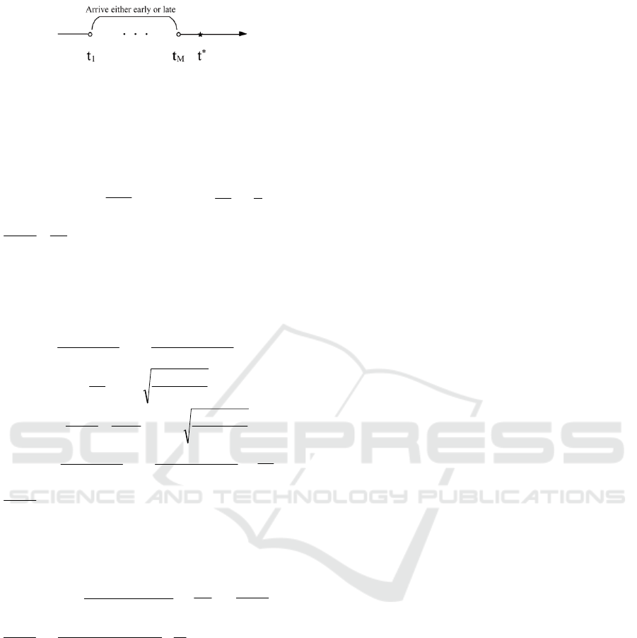
Figure 4: Arrival situation of commuters in peak period in
the third case.
Based on the above formula, we can make a
simple analysis of the change trend of
1
t a n d
TT
C
with
b
value.
When
hMb )1(
2
0 




,
0
2
1
1

db
dt
,
0
2

N
db
dTTC

. So in Scenario 1, the initial time of
peak period
1
t decreases monotonically with the
increase of
b
value, and the total system cost
TT
C
increases monotonically with the increase of
b
value.
When





2
)1)(()1(2 hM
b
hM 



:
b
hM
db
dt
)(2
)1(
1
1





(29)
b
hM
NN
db
dTTC
)(2
)1(
2 








(30)
When





2
)1)(()1(2 hM
b
hM 



,
0
1

db
dt
,
0
db
dTTC
. So in Scenario 2, the initial time of peak
period
1
t decreases monotonically with the increase
of
b
value, and the total system cost
TT
C
increases
monotonically with the increase of
b
value.
When



2
)1)(( hM
b



,
0
1





db
dt
,
0)(
28
)1)((
2
22


 

N
b
NhM
db
dTTC
. So in
Scenario 3, the initial time of peak period
1
t
decreases monotonically with the increase of
b
value, and the total system cost
TT
C
increases
monotonically with the increase of
b
value.
4 CONCLUSIONS
This paper extends the bottleneck model to study the
travel behavior of subway commuters during rush
hours. The extended model takes into account the
situation that passengers have a random delay
T
,
which follows a uniform distribution in the range
bT


0
, to reach their workplace after getting off
the subway. It is shown that with the increase of
b
,
three different scenarios emerge. The start time and
end time of the peak hour, the expected value of travel
cost, and the queuing time have been derived under
the three scenarios. It is shown that the start time of
rush hour monotonically decreases (i.e., the start time
becomes earlier and earlier) and the travel cost
monotonically increases with the increase of
b
.
In our future work, we will consider how to
manage the subway commute under random delay to
lower down the travel cost of commuters.
ACKNOWLEDGEMENTS
The work is funded by the National Key R&D
Program of China (Grant No. 2019YFF0301300).
REFERENCES
Arnott, R., De Palma, A., Lindsey, R., 1990. Economics of
a bottleneck. Journal of Urban Economics. 27 (1), 111–
130.
Arnott, R., De Palma, A., Lindsey, R., 1993. A structural
model of peak-period congestion: a traffic bottleneck
with elastic demand. Am. Econ. Rev. 83,161–179.
Braid, R.M., 1989. Uniform versus peak-load pricing of a
bottleneck with elastic demand. J. Urban Econ. 26 (3),
320–327.
Hai Yang,Yili Tang, 2018. Managing rail transit peak-hour
congestion with a fare-reward scheme. Transp. Res.
Part B. 110, 122-136
Kraus, M., Yoshida, Y., 2002. The commuter’s time-of-use
decision and optimal pricing and service in urban mass
transit. J. Urban Econ. 51 (1), 170–195.
Ling-Ling Xiao,Hai-Jun Huang, Ronghui Liu, 2015.
Congestion Behavior and Tolls in a Bottleneck Model
with Stochastic Capacity. Transportation Science.
49(1), 46-65.
Laih, C., 2004. Effects of the optimal step toll scheme on
equilibrium commuter behaviour. Appl. Econ. 36 (1),
59–81.
Lindsey, R., van den Berg, V.A.C., Verhoef, E.T., 2012. Step
tolling with bottleneck queuing congestion. J. Urban
Econ. 72 (1), 46–59.
Vickrey, W.S., 1969. Congestion theory and transport
investment. Am. Econ. Rev. 59, 251–260.
Yang, H., Meng, Q., 1998. Departure time, route choice and
congestion toll in a queuing network with elastic
demand. Transp. Res. Part B. 32 (4), 247–260.
Zheng Zhu,Xinwei Li,Wei Liu,Hai Yang, 2019. Day-to-day
evolution of departure time choice in stochastic
capacity bottleneck models with bounded rationality
and various information perceptions. Transportation
Research Part E.131.
Effects of Random Delay on Travel Behavior of Subway Commuters during Peak Hour based on Equilibrium Models
123

APPENDIX
The First Train May Arrive Early or
Late, and the Last Train Is Always Late
When





2
)1)(()1(2 hM
b
hM 



, it is also
possible that the commuters taking train
2
~1 m
arrive early or late, and the commuters taking train
Mm ~1
2

always arrive late. In this case, the peak
starts and ends at:

















bhM
hMt
bhM
t
M
)1(2
)1(
)1(2
1
(31)
Since commuters in the first train may be early or
late, and commuters in the tail train are always late,
then:
hMbhM
t
bt
M
)1(
2
)(
)1(
2
0
0
1














(32)
Because
hM )1(
2
)(2









, Scenario 2'
cannot exist.
PMBDA 2021 - International Conference on Public Management and Big Data Analysis
124