
A Modified SAIR Model for the Spread of COVID-19 in China
Yijun Guo
School of Pharmaceutical Sciences, Sun Yat-Sen University, Guangzhou, 510006, China
Keywords: COVID-19 Prediction, Sir Model, Asymptomatic Patients.
Abstract: The study aims to modify the SIR model with consideration of asymptomatic patients for the spread of
COVID-19 in China. The data is obtained from the National Health Commission of the PRC. Data fitting
based on Chinese epidemic data is conducted to find the value of parameters. Besides, sensitivity analysis is
applied on parameters, and the new modified model is compared with model having a similar structure in the
previous study. For further investigation, the basic reproduction number, R
0
, turning point and ratio between
asymptomatic and total infected ones are calculated. The fitting and sensitivity analysis reveals that loss of
immunity, ratio between infection rate of asymptomatic ones and infected ones will not significantly influence
the SAIR model. The analysis results also show that structure of previous model with related infection rates
does not work well on chosen data. On the contrary, transformation rate from asymptomatic ones to infected
patients plays a critical role in the epidemic. mentioned above. Further evaluation shows that it can be used
as a reference for the arrangement of testing. The model can be used to predict the general evolution of the
disease spread. The increase of the transformation rate can alleviate the spread of disease. Transformation rate
can be interpreted as the frequency of testing, which further confirms the necessity of these methods and
provides some application values. The model is plausible but more analysis is still needed to evaluate the
different conditions to apply.
1 INTRODUCTION
COVID-19, a respiratory disease, has caused the
death of 4.29 million people, and approximately 202
million positive cases have been detected from Dec
30th 2019 till Aug 10th 2021(Coronavirus disease
(COVID-19) pandemic, 2021). Vaccination is
considered to be an effective method to suppress the
spread of COVID-19. However, the biosecurity of
vaccination and duration of immunity still need time
to prove (Huang, 2021; Vashishtha & Kumar, 2021).
What's more, the mutation rate of SARS-CoV-2 is
fast and diversified, which can hardly be caught up
by the speed of vaccination development. The
mutation of highly pathogenic strain “Delta” to
“Delta-plus”, or “AY.1” detected in June 2021 in
India brings more challenges (Banerjee et al., 2021).
Until now, we can still assume that stable immunity
against COVID-19 has not been totally built among
people.
Asymptomatic patients with COVID-19 will
unconsciously spread disease to their contacts since
they may not receive diagnosis because they do not
show symptoms (Kronbichler et al., 2020). The
asymptomatic can be divided into two groups, one
will recover without the symptoms, and the other will
show the symptoms and become the normally
assumed “infected people” in epidemiology concepts.
Multiple detection and tracking methods can be
applied to screen out asymptomatic population,
which will promote the performance of isolation,
treatment and other strategies to control the influence
of this group (Chaimayo et al., 2020; Rivett et al.,
2020).
The Susceptible-Infected-Removed (SIR) model
is commonly used in the epidemiological studies and
prediction for outbreak of certain disease (Lounis &
Bagal, 2020). Traditional SIR model divides people
into three groups: the susceptible (S), the infected (I),
and the removed (R). However, the design of
traditional model cannot display the true infected
situation well. Patients who recovered from the
disease can be easily infected again (Abou-Ismail,
2020). Here, we consider the condition that part of
people recovered from disease will not get stable
immunity. We also take asymptomatic patient into
account, since they may have different infected and
recovery rates as the infected ones. In this study, we
Guo, Y.
A Modified SAIR Model for the Spread of COVID-19 in China.
DOI: 10.5220/0011159100003437
In Proceedings of the 1st International Conference on Public Management and Big Data Analysis (PMBDA 2021), pages 197-207
ISBN: 978-989-758-589-0
Copyright
c
2022 by SCITEPRESS – Science and Technology Publications, Lda. All rights reserved
197
evaluate the newly built model and parameters based
on the simulation of R. Besides, by data fitting and
sensitivity analysis, we investigate the role of these
parameters in the model. According to the analysis of
parameters, we further evaluate the strategies that can
be applied to control the disease.
2 SAIR MODEL
2.1 Model Equations
As mentioned above, infected individuals can be
divided into two parts, the infected ones and the
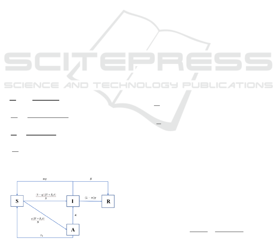
asymptomatic ones. In the SAIR model, the four
groups we concern are S (t) for susceptible, I (t) for
infected, A (t) for asymptomatic and R (t) for
recovered. Figure 1 shows the interrelationships of
these parts.
The model set assumptions as follows: 1)
demographical changes for the asymptomatic, the
susceptible and the recovered are ignored; 2) only
death rate of the infected will be considered here; 3)
part of asymptomatic patients will transform into
infected ones; 4) infected ones and asymptomatic
ones have different infection rate and recovery rate;
5) the total population is denoted by N (t), and
contains four groups, S (t), I (t), A (t) and R (t).
Change of four fractions can be described by the
following differential equations.
=−
(
)
+𝑚𝛾𝐼 +𝛾
𝐴 (1)
=
(
)(
)
−
(
𝛾
+𝜅
)
𝐴 (2)
=
(
)
−
(
𝛾+𝜇
)
𝐼+ 𝜅𝐴 (3)
=𝛾𝐼
(
1−𝑚
)
+ 𝜇𝐼 (4)
𝑁 =𝑆+𝐼+𝐴+𝑅=1 (5)
Figure 1: Flow chart of the SAIR model.
Parameters above in this model are positive and
can be interpreted as follows:
• β is the infection rate of infected individuals;
• β
1
is the infection rate of asymptomatic
individuals;
• γ is the recovered rate of infected individuals;
• γ
1
is the recovery rate of asymptomatic ones;
• μ is the death rate of infected ones;
• κ is the possibility for asymptomatic patients
to become infected ones at a certain time,
which means they will show the symptoms or
be regarded as infected by certain criteria;
• q is the possibility for susceptible people who
contact with asymptomatic ones and infected
ones to become infected ones, while 1-q
means the possibility to become
asymptomatic ones;
• m means the possibility for recovered
asymptomatic people to become susceptible
again. They are assumed to have no stable
immunity.
2.2 Analysis of Mathematical Model
2.2.1 Basic Reproduction Number
The basic reproduction number, R
0
of the SAIR
model was calculated using the next generation
matrix methods (Diekmann et al., 2010). To calculate
the basic reproductive number, the approximation of
S (t) could be N when t ≈ 0. Based on Eq. (1)-(5), Eq.
(2) and Eq. (3) could be expressed as:
=
(
1−𝑞
)(
𝛽𝐼+ 𝛽
𝐴
)
−
(
𝛾
+𝜅
)
𝐴
=𝑞
(
𝛽𝐼+ 𝛽
𝐴
)
−
(
𝜇+ 𝛾
)
𝐼+ 𝜅𝐴
(6)
From Eq. (6) we can get the matrix
𝑋=
()
()
=
(
)(
)
(
)
+
(
)
(
)
=
𝐹
,
(
𝐴,𝐼
)
+ 𝑉
,
(
𝐴,𝐼
)
(7)
𝐹= 𝐽𝑎𝑐𝑜𝑏𝑖𝑎𝑛(𝐹
,
(
𝐴,𝐼
)
)=
(
1−𝑞
)
𝛽
(
1−𝑞
)
𝛽
𝑞𝛽
𝑞𝛽
(8)
𝑉= 𝐽𝑎𝑐𝑜𝑏𝑖𝑎𝑛(𝑉
,
(
𝐴,𝐼
)
)=
𝛾
+𝜅 0
−𝜅 𝜇 + 𝛾
(9)
R
0
can be calculated as the eigenvalues of 𝐹𝑉
:
𝑅
=
(
)
+
(
)
(
)
(
)
(10)
R
0
is normally used to evaluate whether the
outbreak of disease will happen. When R
0
≤1, the
PMBDA 2021 - International Conference on Public Management and Big Data Analysis
198
system is supposed to have disease-free equilibrium
and the number of infected people will decrease. On
the contrary, endemic equilibrium will exist when R
0
> 1. An increase of μ and γ leads to decrease of R
0
,
which leads to the elimination of disease. In the
fitting part, we will discuss influence of value of κ to
R
0
. Parameter m seems to have little influence on
basic reproduction number.
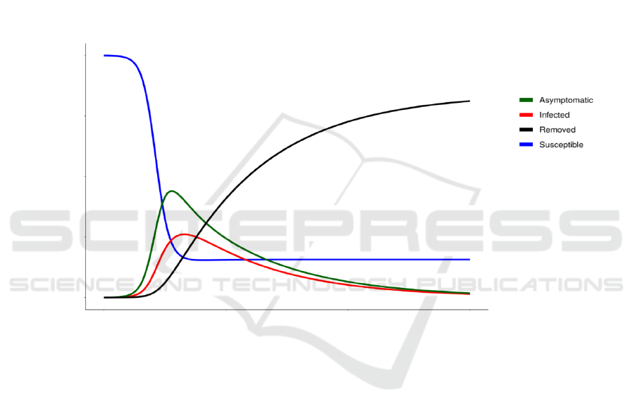
2.2.2 Simulation of SAIR Model
To find numerical solutions of the model, we set the
following initial values for parameters:
𝑁
(
0
)
=1,𝑆 (0) = 𝑁 (0) − 𝐼 (0),
𝐼 (0)=0.0005,𝐴 (0)=0,
𝛽 = 0.3,𝛽
= 0.5,𝛾 =1/7,𝛾
=1/21,
𝜇 = 0.002,𝑚 =0.6, 𝑞 = 0.2,𝜅 = 1/14
By introducing the normalization condition,
where N is set to be 1, the effect of the total population
on the modeling outcome can be eliminated to some
extent. The time evolution of four fractions is
displayed in Figure 2.
Figure 2: Numerical solutions for fractions of susceptible, asymptomatic, infected, and recovered in the SAIR model.
Parameter values: β =0.3, β
1
= 0.5, γ =1/7, γ
1
=1/21, μ = 0.002, m =0.6, q = 0.2, κ = 1/14. Initial values for fractions: N (0) =
1, S (0) = N (0) - I (0), I (0) = 0.0005, A (0) = 0.
As for the set of initial values of parameters, we
initially assume asymptomatic ones will have
stronger infection ability than infected ones because
infected ones are more probable to be isolated. People
with a certain knowledge of the disease will also keep
distance from symptomatic ones. Recovery rate
represents reciprocal of time needed for patients to
recover. Here we set γ and γ
1
as 1/7 and 1/21
respectively according to the previous research
(Neves & Guerrero, 2020). Some of the
asymptomatic people will get normal unconsciously
without showing symptoms in this model. The other
part of the asymptomatic population will become
infected ones. Transformation rate without inference
can be assumed as length of incubation period. Since
most countries set the quarantine for 14 days, we can
primarily set κ as 1/14 (Gaeta, 2020). In that case, the
transformation rate, κ, is primarily set to be 1/14 days
-
1
. And the death rate is set according to the analysis
of death cases in real data, which will be introduced
in the data fitting part. Since the number of
asymptomatic behind the confirmed cases is usually
larger than confirmed number, q is set to be lower
than 0.5 to simulate that condition.
0 50 100 150
0.00 0.25 0.50 0.75 1.00
Time
(
da
y)
Individuals
A Modified SAIR Model for the Spread of COVID-19 in China
199

2.2.3 Conditions for Elimination of Disease
The total infected ones can be represented as I (t) +A
(t), and disease starts to eliminate when:
()
<0 (11)
The number of asymptomatic patients is much
larger than infected ones and they can transform into
infected ones according to the model. The most
important is that A (t) has a stronger infection ability
compared with I (t) based on assumptions of this
model. For the reasons above, we assume I (t) / A (t)
≈ 0, and we use A (t) to substitute whole infected
people. We can get:
𝑆
(
𝑡
)
<
(
)
()(
)
(12)
Combined with Eq. (2) and Eq. (11), Eq. (12) can
be transformed into:
𝑆
(
𝑡
)
<
()(
)
≈
()
(13)
We can see that when asymptomatic patients play
a critical role during the epidemic of the disease, the
elimination of total infected ones will start when S (t)
reaches
. Recovery rate and infection rate of
asymptomatic patients decide the peak of disease.
However, one thing that should be paid attention to is
that conclusion above can only be achieved when A(t)
plays main role in the system, so the value of q should
be small.
2.2.4 Comparison between Modified SAIR
Model and SAIR Model in Previous
Study
In the SAIR model sourced from previous study
(Neves & Guerrero, 2020), an SAIR model was built:
=−𝛽
𝑆(𝐼+ 𝜇𝐴) (14)
=𝛽
(1 −𝜉)𝑆
(
𝐼+𝜇𝐴
)
−𝛾
𝐴 (15)
=𝛽
𝜉𝑆
(
𝐼+𝜇𝐴
)
−𝛾
𝐼 (16)
=𝛾
𝐼 (17)
=𝛾
𝐴 (18)
𝑵 =𝑺+𝑰+𝑨+𝑹
𝒔
+𝑹
𝜶
(19)
We can call this model P, and the new model in
this paper is model M. In model P, γ
α
and γ
s
denotes
recovery rates of asymptomatic ones and infected
ones. Infection rate of infected patients and
asymptomatic patients are represented by β
0
and μβ
0
.
Table 1 shows a simple comparison of the two
models.
Table 1: Comparison of two SAIR models.
Items Model M Model P
Variables 4 5
Basic reproduction number
(
1−𝑞
)
𝛽
𝛾
+𝜅
+
𝛽(𝜅 +𝛾
𝑞)
(
𝛾
+𝜅
)
(
𝜇+𝛾
)
𝛽
[
𝜉
𝛾
+
𝜇
(
1−𝜉
)
𝛾
]
Death rate μ None
Immunity duration Unstable Stable
Infection rates
A (t) : 𝛽
, I (t) : 𝛽 A (t) : 𝜇𝛽
, I (t) : 𝛽
Relations between two infection rates Unrelated Related
S (t) for elimination of disease
𝛾
+𝜅
𝛽
(
1−𝑞
)
𝛾
𝛽
(1 − 𝜉)𝜇
Transformation rate from A (t) to I (t)
𝜅
None
From the comparison we can see main differences
between the two models. Model P does not consider
death rate (μ in model M), transformation rate (κ) or
unstable immunity (m). As for infection rates, β and
β
1
in Model M are not related as model P.
PMBDA 2021 - International Conference on Public Management and Big Data Analysis
200
3 FITTING THE EPIDEMIC
DATA OF COVID-19 ON SAIR
MODEL
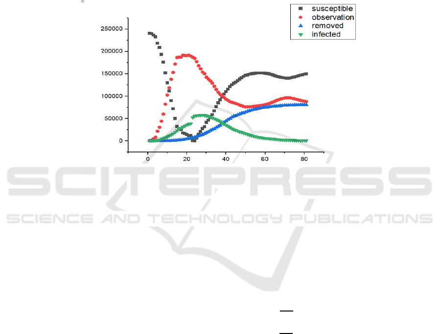
3.1 Fitting the Epidemic Data in China
Data used for fitting is from National Health
Commission of the PRC (Official report of COVID-
19, 2021). Present confirmed cases, death cases,
recovered cases and the number of people under
observation are reported every day. Observation
cases in China include people who show slight
symptoms and people who are tracked to have contact
with infected ones. Figure 3 shows evolution of four
kinds of data from 21
st
Jan, 2020 to 10
th
Apr, 2020.
We choose the initial stage of the COVID-19 in China
because isolation strategy worked well later, which
significantly influenced the spread of disease.
Timeframe from 21
st
Jan to 10
th
Apr includes just
single peak of confirmed cases, which is also
compatible with assumption of model M.
Figure 3: Epidemic data in China from 21
st
Jan, 2020 to 10
th
Apr, 2020 by National Health Commission of the PRC. N is set
to be 241835.
We can see from Figure 3 that both removed and
infected cases finally reach a plateau. Infected cases
have a single peak during the timeframe. However,
the number of cases under medical observation has a
small fluctuation after the peak. This group of
population may be influenced by a newly discovered
case or some policies.
For the total size of population, N, we cannot
choose population of the full country as N
(Ahmetolan et al., 2020), because epidemic of SARS-
CoV-2 in China is highly heterogeneous. The max
sum of confirmed cases (55748), cumulative death
cases (1380), cumulative recovery cases (6732) and
present observation cases (177984) appeared on 13
th
Feb 2020, which can be used to substitute N at initial
stages. Asymptomatic ones are hard to be detected
and reported. We can consider the worst condition
that all of the people who show slight symptoms or
have contact with the infected ones could be
asymptomatic. Here, we assume number of
observation cases is approximate to asymptomatic
ones. N’ denotes the population at initial stage, which
is 241835. Confirmed cases reported by government
can be treated as infected ones in this model. Death
ones can be precisely estimated by death cases
reported. Here, we can divide R into two parts, one is
for the death (R
d
), and the other is for the recovered
ones (R
a
). So Eq. (4) could be transformed as follows:
=𝜇𝐼 (20)
=
(
1−𝑚
)
𝛾𝐼 (21)
To calculate μ, we use R to apply regression
diagnosis on reported daily infected cases and daily
death cases to find if linear regression can be used on
true data. Figure 4 shows diagnosis results regarding
to normality, linearity, homoscedasticity and simple
observation points. We can see from the result that it
number of death cases is linear with confirmed cases,
which reflect the relationship in Eq. (20). So here, we
could use true data to calculate μ. μ is calculated to be
0.002 by R.
Tim
e
(d
a
y)
Individuals
A Modified SAIR Model for the Spread of COVID-19 in China
201
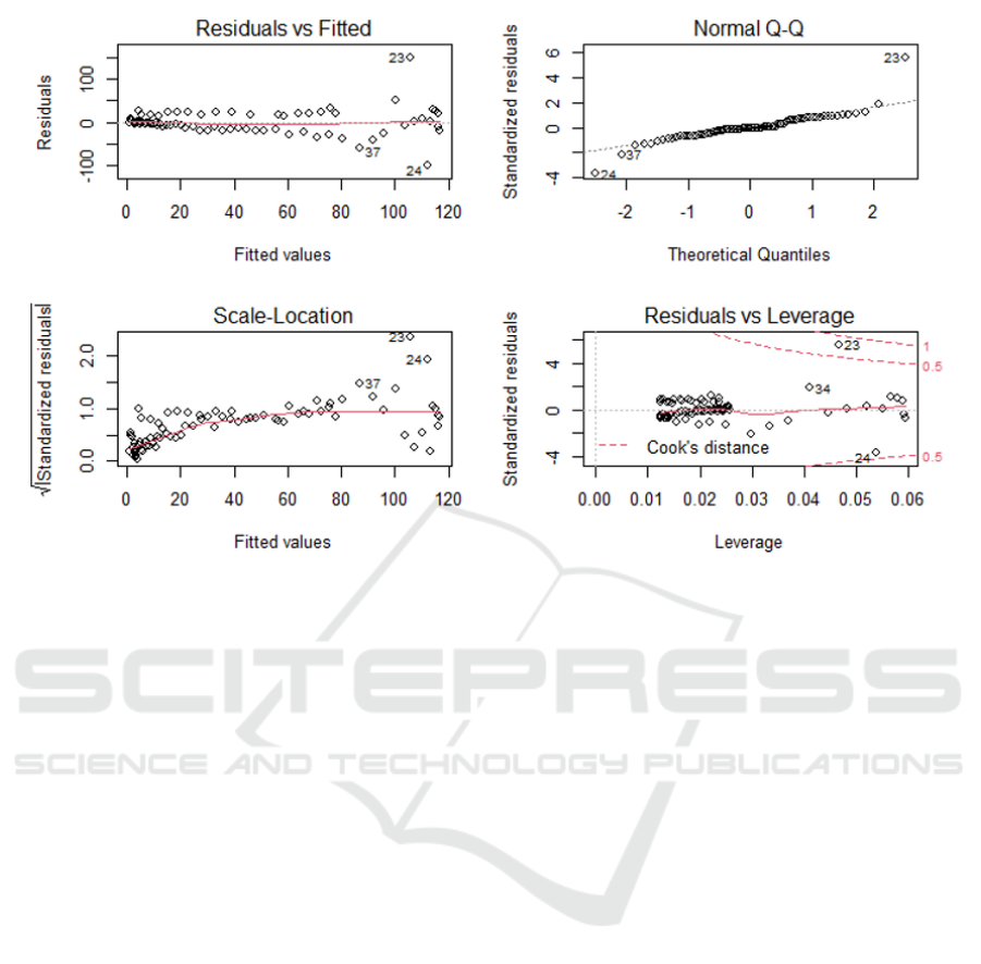
Figure 4: Diagnosis of linear regression of daily infected cases and daily death cases. (A) Plot of residuals vs fitted. (B)
Normal Q-Q plot. (C) Scale-Location plot. (D) Plot of residuals vs leverage.
We use confirmed cases to estimate these
parameters here because death cases and
asymptomatic cases were proved to be proportional
to infected cases (Ahmetolan et al., 2020; Grunnill,
2018). The cost function between predicted data and
true data can be described as follows (Ianni & Rossi,
2020).
𝐽
𝜃
=
∑
𝐼𝑡
;𝜃
−𝑁
(
𝑡
)
(22)
𝐽
𝜃
=
∑
𝐴𝑡
;𝜃
−𝑁
(
𝑡
)
(23)
𝐽
𝜃
=
∑
𝐷𝑡
;𝜃
−𝑁
(
𝑡
)
(24)
𝑁
,,
(
𝑡
)
represents true data cases in the time
frame till 𝑡
. 𝜃
= {β, β
1
, γ, γ
1
, m, μ, κ, q, N, I (0), A
(0), 𝑅
(0)}. The value of parameters can be
estimated based on the least cost. Initial values of
parameters are set in Figure 2. We set initial values
according to epidemic data at the start of time frame:
𝑁
(
0
)
=92388,𝑆 (0) = 𝑁 (0) − 𝐼 (0),𝐼(0)
=291,𝐴(0)=922
The fitting of the data is conducted by FME
package in R.
Eq. (22-24) are used to fit the data, the result is as
follows:
(
A
)
(
B
)
(
C
)
(
D
)
PMBDA 2021 - International Conference on Public Management and Big Data Analysis
202
(A)
(B)
(C)
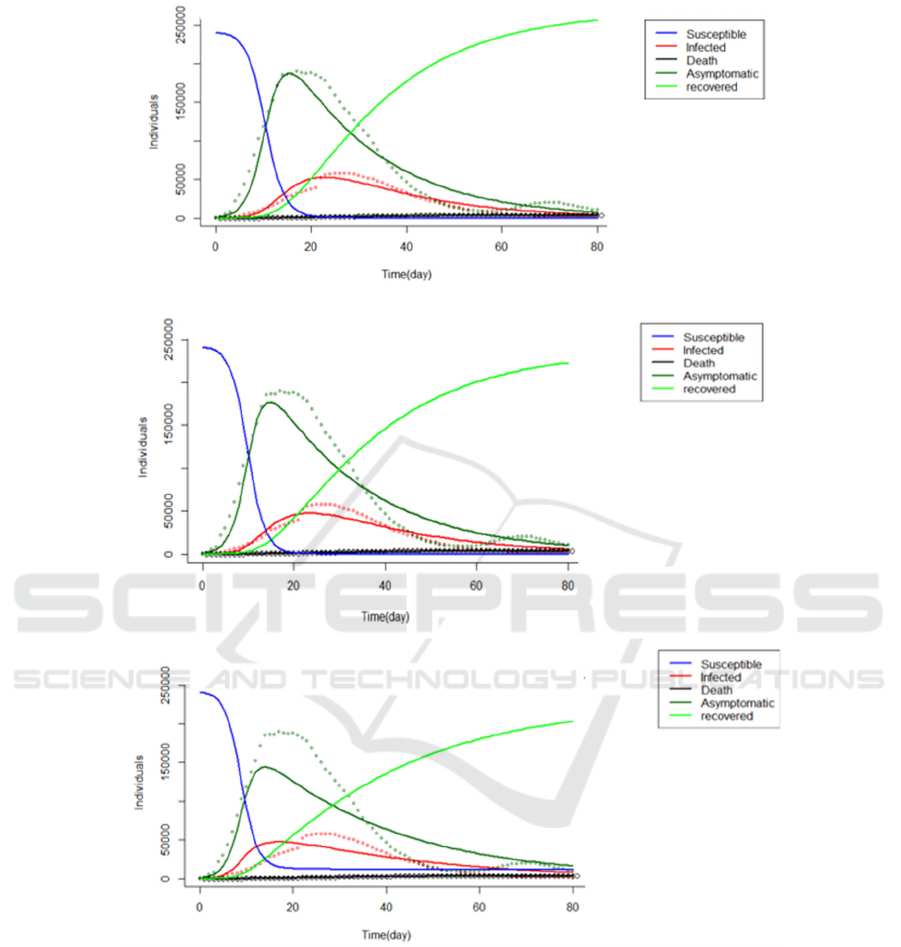
Figure 5: Fitting of I (infected), A (asymptomatic) and R
d
(death) on Chinese data from 21
st
Jan, 2020 to 10
th
Apr, 2020. (A)
Fitting without related infection rate. (B) Fitting with related infection rate. (C) Fitting with several selected parameters.
We can see from Figure 5 (A) that the model fits
data well at the initial stage but not very well around
the peak. The model can depict the general changing
trend of five parts. By investigating the parameters,
we find that the fitting result is not compatible with
our assumptions. In our assumptions of model,
infection rate of infected ones should be lower than
asymptomatic ones. So here, we relate β with β
1
by n
(β = nβ
1
, 0< n <1) like model P, so that we could
guarantee β
1
is always larger than β. n is initially set
to be 0.6. In this way, we could also find whether the
relationship between infection rates matters in this
model. The fitting result is showed in Figure 5 (B)
and Table 2. There is no significant change between
results. From the fitting results, we can conclude that
ratio between β and β
1
does not play a critical role in
the fitting of Chinese data.
A Modified SAIR Model for the Spread of COVID-19 in China
203

Table 2: Comparison of parameters with and without fixed parameters.
Parameters
Value
Original parameter Related infection rate Selection of parameters
β 0.999 / 0.999
γγ 0.124 0.125 0.119
β
1
0.497 0.543 0.564
γ
1
1.40*10
-7
8.93*10
-8
4.76*10
-2
(fixed)
κ
4.55*10
-2
4.57*10
-2
4.36*10
-2
q
4.78*10
-7
3.31*10
-7
0.200 (fixed)
m
1.32*10
-6
8.71*10
-7
0.600 (fixed)
μ
2.12*10
-3
2.12*10
-3
2.12*10
-3
n / 0.999 /
3.2 Sensitivity Analysis of Parameters
Sensitivity analysis is conducted on parameters in the
first column in Table 2 (β ≠ nβ
1
) to show the influence
of parameters (Table 3). m, γ
1
and q seem to have little
influence on this dataset, which confirmed the
parameter calculation results in Table 2. We choose
parameters except m, γ
1
and q as parameters to fit; the
results are in Figure 5 (C) and Table 2. Interestingly,
we find that the fitting result is not as well as the first
two sets of parameters. From the original plot, we can
conclude that the source of data lead to that result.
Since data used to describe asymptomatic is the
number of people under medical observation, so there
is a time lag between growth of A (t) and I (t). m, γ
1
and q might work here to guarantee the time lag. If
the model fitting is conducted without m, γ
1
or q,
growth of A (t) will be synchronized with growth of I
(t) as Figure 5 (C) shows.
Sensitivity also shows that κ has a great impact on
model and almost remain unchanged when we change
the design of model as above. κ represents rate of
asymptomatic ones to become infected ones. The
value of κ is about 0.0457, which means that time
need for asymptomatic ones to become infected ones
is about 22 days (1 / 0.0457 day-1).
Table 3: Sensitivity analysis of parameters.
Parameter
Item
value L1 L2 Mean Min Max
β 0.999 0.120 0.178 0.0450 -0.0850 0.553
γ 0.124 0.555 0.749 -0.547 -1.49 0.0168
β
1
0.497 0.528 0.779 0.183 -0.388 2.55
γ
1
2.33*10
-7
3.12*10
-7
4.53*10
-7
-2.66*10
-7
-1.31*10
-6
1.32*10
-7
κ
4.55*10
-2
0.872 1.15 -0.317 -3.18 1.01
q
8.84*10
-7
1.61*10
-6
2.73*10
-6
6.07*10
-7
-1.06*10
-6
9.92*10
-6
μ 2.12*10
-3
0.331 0.567 0.320 -0.0254 0.999
m 2.34*10
-6
2.10*10
-6
3.22*10
-6
2.10*10
-6
0.000 9.06*10
-5
3.3 Epidemic Items and Strategies to
Alleviate COVID-19 based on Κ
Several items regarding epidemic evolution are
calculated with the original set of parameters. The
results are displayed in Table 4. R
0
is 18.8 (R
0
> 1),
which indicates that the outbreak of disease is still
potential without inference. R
0
also considers the
existence of asymptomatic patients at the end of time
frame. Though the number of infected ones has been
eliminated, asymptomatic patients may still bring
fluctuations. S (t) / N can work as evidence of the
turning point of disease. Value of S (t) / N indicates
that the turning point of disease is approximately on
the 20th day. Figure 5 further confirmed the
prediction of turning point. A (t) / (I (t) +A (t)) (Figure
6 (A)) indicates that ratio between asymptomatic ones
and total infected ones will finally reach the plateau
(0.641), which could be used to predict fractions and
number of asymptomatic ones.
PMBDA 2021 - International Conference on Public Management and Big Data Analysis
204
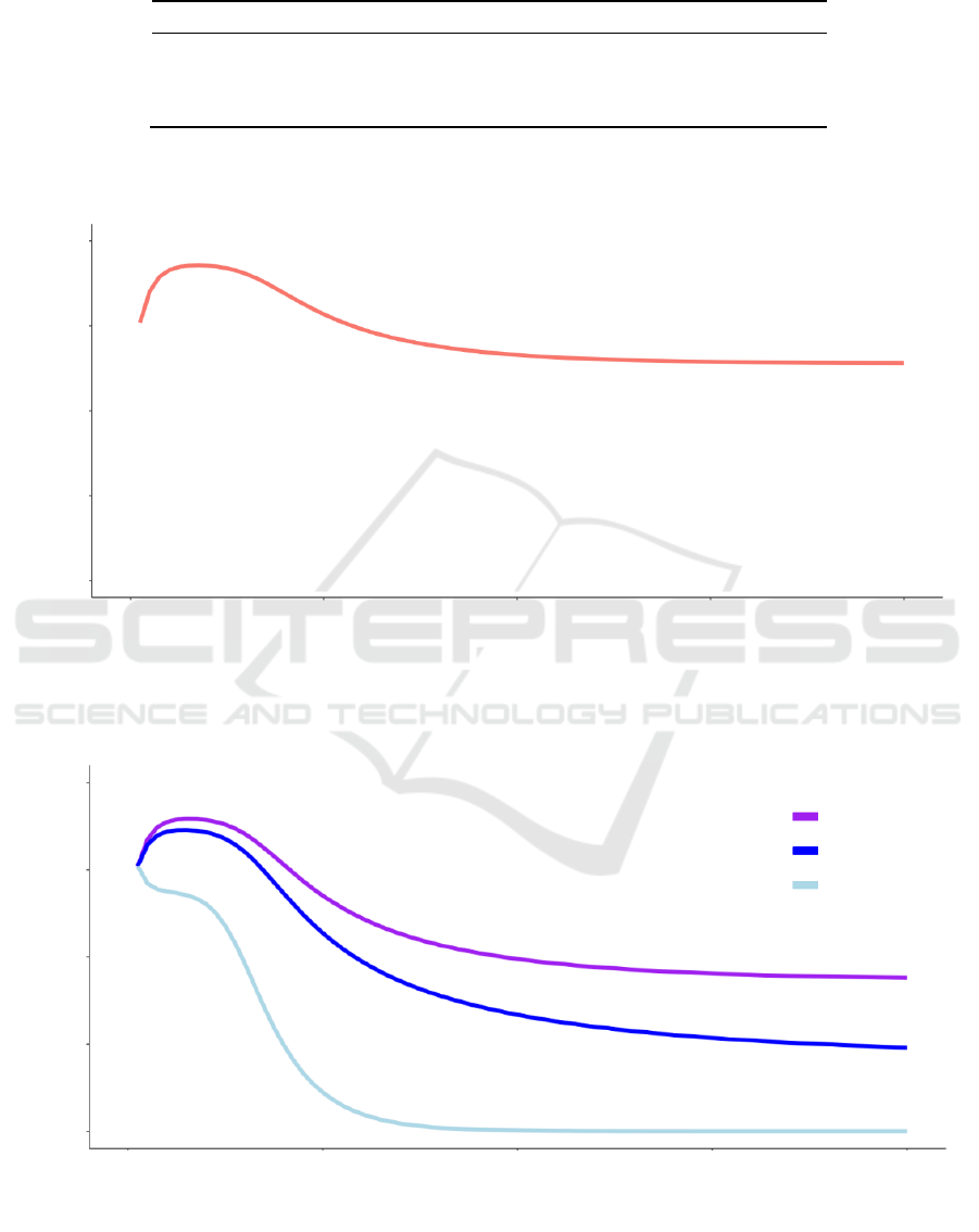
Table 4: Several epidemic items calculated by model.
Item Value
R
0
18.8
S (t) / N 0.0915
A (t) / (I (t) +A (t)) 0.641
(A)
(B)
Figure 6: Ratio of A (t) / (I (t) +A (t)). (A) A (t) / (I (t) +A (t)) calculated by original parameters in Table 2. (B) A (t) / (I (t) +A
(t)) under different values of κ (1/14, 1/10,1/3).
0.00 0.25 0.50 0.75 1.00
0 20 40 60 80
Time
(
da
y)
A
(
t
)
/
(
I
(
t
)
+A
(
t
))
A
(
t
)
/
(
I
(
t
)
+A
(
t
))
0 20 40 60 80
0.00 0.25 0.50 0.75 1.00
Time
(
da
y)
κ =1/14
κ =1/10
κ =1/3
A Modified SAIR Model for the Spread of COVID-19 in China
205
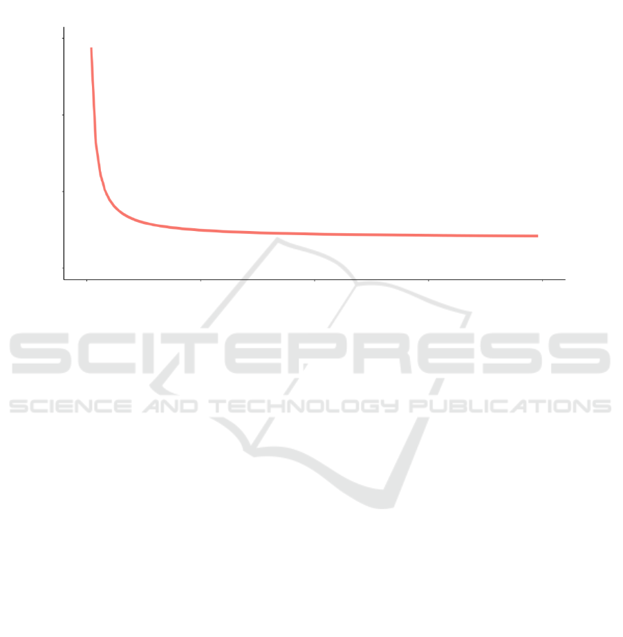
Since the role of κ is confirmed by sensitivity
analysis, we further evaluate how R
0
, S (t) and A (t) /
(I (t) +A (t)) can be influenced by κ. Here, changes of
A (t) / (I (t) +A (t)) and R
0
under different values of κ
are shown in Figure 6 (B) and Figure 7. The results
show that plateau proportion of asymptomatic will
decrease. Furthermore, R
0
become smaller if we
change the value of κ from 0 to 1 based on this set of
parameters. From Eq. (13) we can know that S (t) will
increase with the increase of κ.
Figure 7: R
0
calculated by original parameters under different values of κ (0 <κ< 1)
To sum up, the burden of asymptomatic patients
and the spread of disease can be alleviated by
regulating of κ. Several methods can be applied based
on interpretation of κ such as nucleic acid
amplification testing (NAT) like oropharyngeal (OP)
(Rivett et al., 2020), tracking or isolation. If we
assume κ as the frequency of NAT, we can get more
information for reference from κ. We can see in
Figure 7 that the decrease of R
0
gradually gets slower
after κ is smaller than certain value. The value in this
system is approximate 0.25. Figure 6 (B) also
confirms that when κ gets close to 1/3, there will not
be an initial increase of A (t) / (I (t) +A (t)), and the
ratio will quickly get down. From the above results,
we can infer that the proper testing frequency can be
set as once per three days or four days in the spread
condition of China. If there is a lack of source for
frequent testing, evaluations regarding κ can also be
taken as a reference for testing arrangement.
4 CONCLUSION
For the consideration of asymptomatic patients, we
build new SAIR model to better fit the real condition
of the disease. Asymptomatic patients will keep
infecting the susceptible because they show no
syndrome and will not be detected, isolated and
treated. So here, the model is modified to find the
influence of this group. And previous study about
model with a similar structure is used for comparison
in this study (Neves & Guerrero, 2020).
Our model adds the assumption that the infected
ability of asymptomatic patients will not be related to
the infected ability for infected groups. We also
evaluate the role of transformation rate from the
asymptomatic to the infected. And immunity will not
be built on all people who recovered. By comparison
with previous model, we also find that it is too haste
to just relate two infection rates by a simple
coefficient (β = nβ
1
) because of choice of data
representing asymptomatic population. Data
evolution from hospital regarding people under
medical observation may have a time lag of change
on infected people. So, if we choose medical
observation data as asymptomatic ones, two
parameters cannot be simply related when fitting.
From the fitting results and sensitivity analysis we
can conclude that parameters regarding part
immunity dose not significant the fitting results.
0.00 0.25 0.50 0.75 1.00
0
20 40 60
R
0
κ
PMBDA 2021 - International Conference on Public Management and Big Data Analysis
206

Transformation rate plays a critical role in the
evolution of disease. Here, we assume κ can be
interpreted as frequency of NAT. We find that several
epidemic items can be calculated to display influence
of κ on testing arrangement.
The model used here is a simple design of SAIR
model. Focusing on the influence of asymptomatic
ones, it does not take into account of multiple factors.
In other studies, spread in different communities,
countries and between different groups of people, for
example, the elder and teenagers are evaluated
(Cooper et al., 2020; Harris, 2020; Purkayastha et al.,
2021). Some models also considered the removed or
isolated ones which will make the total population
heterogeneous (Maheshwari & Albert, 2020). In the
more sophisticated design, recovered and infected
groups could be divided into more groups to improve
the applicability of model (Tomochi & Kono, 2021).
In that case, the model still has a large potential to
develop and attain higher application value.
REFERENCES
Abou-Ismail A. (2020). Compartmental Models of the
COVID-19 Pandemic for Physicians and Physician-
Scientists. SN Compr Clin Med, 1-7.
Ahmetolan S., Bilge A. H., Demirci A., Peker-Dobie A., &
Ergonul O. (2020). What Can We Estimate From
Fatality and Infectious Case Data Using the
Susceptible-Infected-Removed (SIR) Model? A Case
Study of Covid-19 Pandemic. Front Med (Lausanne),
7, 556366.
Banerjee I., Robinson J., Asim M., & Sathian B. (2021).
Mucormycosis and COVID-19 an epidemic in a
pandemic? Nepal J Epidemiol, 11(2), 1034-1039.
Chaimayo C., Kaewnaphan B., Tanlieng N., Athipanyasilp
N., Sirijatuphat R., Chayakulkeeree M., . . .
Horthongkham N. (2020). Rapid SARS-CoV-2 antigen
detection assay in comparison with real-time RT-PCR
assay for laboratory diagnosis of COVID-19 in
Thailand. Virol J, 17(1), 177.
Cooper I., Mondal A., & Antonopoulos C. G. (2020). A SIR
model assumption for the spread of COVID-19 in
different communities. Chaos Solitons Fractals, 139,
110057.
Coronavirus disease (COVID-19) pandemic. (2021).
Retrieved 10 Aug from
https://www.who.int/emergencies/diseases/novel-
coronavirus-2019.
Diekmann O., Heesterbeek J. A., & Roberts M. G. (2010).
The construction of next-generation matrices for
compartmental epidemic models. J R Soc Interface,
7(47), 873-885.
Gaeta G. (2020). Social distancing versus early detection
and contacts tracing in epidemic management. Chaos
Solitons Fractals, 140, 110074.
Grunnill M. (2018). An exploration of the role of
asymptomatic infections in the epidemiology of dengue
viruses through susceptible, asymptomatic, infected
and recovered (SAIR) models. J Theor Biol, 439, 195-
204.
Harris J. E. (2020). Data from the COVID-19 epidemic in
Florida suggest that younger cohorts have been
transmitting their infections to less socially mobile
older adults. Rev Econ Househ, 1-19.
Huang P. H. (2021). COVID-19 vaccination and the right
to take risks. J Med Ethics.
Ianni A., & Rossi N. (2020). Describing the COVID-19
outbreak during the lockdown: fitting modified SIR
models to data. Eur Phys J Plus, 135(11), 885.
Kronbichler A., Kresse, D., Yoon, S., Lee, K. H.,
Effenberger, M., & Shin, J. I. (2020). Asymptomatic
patients as a source of COVID-19 infections: A
systematic review and meta-analysis. Int J Infect Dis,
98, 180-186.
Lounis M., & Bagal D. K. (2020). Estimation of SIR
model's parameters of COVID-19 in Algeria. Bull Natl
Res Cent, 44(1), 180.
Maheshwari P., & Albert R. (2020). Network model and
analysis of the spread of Covid-19 with social
distancing. Appl Netw Sci, 5(1), 100.
Neves A. G. M., & Guerrero G. (2020). Predicting the
evolution of the COVID-19 epidemic with the A-SIR
model: Lombardy, Italy and São Paulo state, Brazil.
Physica D, 413, 132693.
Official report of COVID-19. (2021).
http://www.nhc.gov.cn/xcs/yqtb/list_gzbd.shtml
Purkayastha S., Bhattacharyya R., Bhaduri R., Kundu R.,
Gu X., Salvatore M., . . . Mukherjee B. (2021). A
comparison of five epidemiological models for
transmission of SARS-CoV-2 in India. BMC Infect Dis,
21(1), 533.
Rivett L., Sridhar S., Sparkes D., Routledge M., Jones N.
K., Forrest S., . . . Collaboration C.-N. C.-B. (2020).
Screening of healthcare workers for SARS-CoV-2
highlights the role of asymptomatic carriage in
COVID-19 transmission. Elife, 9.
Tomochi M., & Kono M. (2021). A mathematical model for
COVID-19 pandemic-SIIR model: Effects of
asymptomatic individuals. J Gen Fam Med, 22(1), 5-
14.
Vashishtha V. M., & Kumar P. (2021). Development of
SARS-CoV-2 vaccines: challenges, risks, and the way
forward. Hum Vaccin Immunother, 17(6), 1635-1649.
A Modified SAIR Model for the Spread of COVID-19 in China
207
