Research on Annual Runoff Forecast of Shaanxi Section of Hanjiang

River based on Multi-model

Shuni He

, Na Wei

*, Linshun Cao

, Zhi Zhang

, Shaofei Zhang

, Feng Yang

and Yating Gao

State Key Laboratory of Eco-hydraulics in Northwest Arid Region, Xi’an University of Technology, Xi’an, Shaanxi

710048, China

Hanjiang-to-Weihe River Valley Water Diversion Project Construction Co., LTD., Shananxi Province, China

Jiangxi Wuda Yangfan Technology Co., Ltd, Nanchang, Jiangxi 330029, China

Keywords: Runoff Prediction,

ARIMA model, MGF model, Grey dynamic model, DenseNet model, Hanjiang River

Abstract: Because of its strong non-stationary and nonlinear characteristics, the runoff series bring serious challenges

to the accurate and reasonable prediction of runoff. In the past, the research direction of runoff prediction is

mainly the improvement of a single model or mixed model prediction, which often ignores the model’s

applicability to the actual situation. From the perspective of multiple models, based on the runoff series data

of Yangxian Station in Shaanxi Section of Han River, this paper adopts the ARIMA model, the MGF model,

the Grey dynamic model and the DenseNet model to forecast the annual runoff of Yangxian Station. The

prediction results are compared and analyzed to select the model most suitable for Yangxian Station among

the four models. The results show that the DenseNet model is the most suitable for the runoff prediction

activities of the selected watershed. Through the applicability analysis of runoff prediction model, a

scientific and reliable runoff prediction can be obtained, which provides a scientific basis for water

resources management and allocation, water resources development and utilization.

1 INTRODUCTION

In recent years, human activities have led to

significant climate change, changes in precipitation

forms, and changes in natural watershed

environment, which makes the change of runoff

more complex (Lei et al., 2003). The prediction of

runoff series becomes more and more difficult.

Under the conditions of existing station network,

instruments and equipment and observation

technology, the temporal and spatial changes of

various information are difficult to reflect. In

addition, affected by objective conditions such as

natural factors, it is bound to cause measurement

errors of various information. There are many

research results of the existing runoff prediction

models, but different models have their own

applicability

(Liang et al., 2020). When predicting

the runoff of the basin, the most appropriate model is

selected from different models to obtain higher

runoff prediction accuracy, which has important

practical significance for accurately predicting the

runoff and is also a problem to be solved in

Hydrological Prediction.

There are many uncertainties and complexities in

runoff time series. At present, people mostly realize

runoff prediction through various hydrological model

methods, including time series prediction model,

nonlinear model and prediction model based on

intelligent algorithm (Labat et al., 2004; Li J et al.,

2008). Time series analysis (Hsu et al., 1995; Dutta et

al., 2012) is an earlier and more mature analysis

method. It studies the change law of prediction with

time and establishes a time series prediction model to

predict. For example, ARIMA model proposed by

box and Jenkins (Du & Ma, 2018; Liu, 2011; Sun et

al., 2013). The mean generating function model

proposed by Wei Fengying et al (Wei & Cao, 1990).

Because the runoff variation characteristics often

show highly nonlinear characteristics, nonlinear

models appear, such as the Grey prediction model

based on Grey system theory (Liu & Yang, 2015;

Deng, 1982a; Deng, 1982b). With the development of

computer technology and mathematical theory,

intelligent algorithms have also been applied to

runoff prediction, such as machine learning, data

mining and so on. For example, DenseNet model, a

machine learning model based on neural network

He, S., Wei, N., Cao, L., Zhang, Z., Zhang, S., Yang, F. and Gao, Y.

Research on Annual Runoff Forecast of Shaanxi Section of Hanjiang River Based on Multi-model.

In Proceedings of the 7th International Conference on Water Resource and Environment (WRE 2021), pages 377-388

ISBN: 978-989-758-560-9; ISSN: 1755-1315

377

theory (Gu, 2008).

There are many models for runoff prediction, but

the characteristics and emphases of different

prediction models are different, and the applicable

conditions are different. There is no best model for

watershed runoff prediction, only suitable models. In

addition, the prediction results of a single prediction

model are lack of comparison, so it is difficult to

obtain accurate and satisfactory results. Therefore, in

the runoff prediction of the basin, it is necessary to

comprehensively compare the prediction results of

different models in order to select a more appropriate

prediction model. From the perspective of multi

model, taking Yangxian station in Shaanxi section of

Hanjiang River as the representative station, this

study uses ARIMA model, MGF model, Grey

dynamic model and DenseNet model to predict the

annual runoff. The results are compared, in order to

select the most suitable runoff prediction model for

Shaanxi section of Hanjiang River.

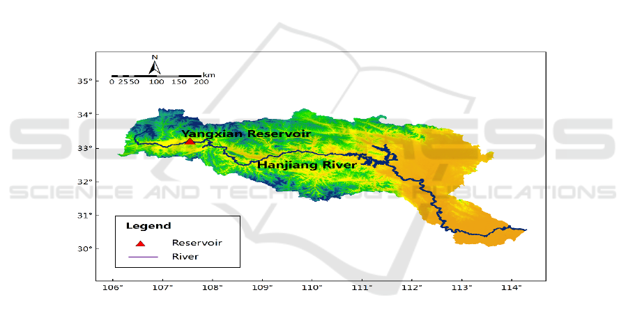
2 STUDY AREA AND DATA

The Han River is the largest tributary of the Yangtze

River, also known as the Hanshui, originating from

Panzhong Mountain in Ningqiang County, Shaanxi

Province. The main stream of the Han River is 1,577

km in length, with a drainage area of 159,000 km².

The section from the source of the upper reaches of

the Han River to the Baihe River belongs to Shaanxi

Province, with a total length of 652 km and a

catchment area of 59,100 km², accounting for about

33% of the total area of Shaanxi Province. The water

volume of this area accounts for about 66.7% of the

entire Shaanxi province, and the river narrow here,

the water level drop is large and the water energy

resources are abundant (Xiong & Chen, 1987).

Yangxian Station on Shaanxi section of Han River at

Daqiaotou, Chengguan Town, Yangxian County, is

an important national control station with a

catchment area of 14,484 km² and a distance of

1,316 km from the estuary (Figure 1).

Figure 1: location of Yangxian station in Shaanxi section of Hanjiang River.

Due to the strong and ever-changing role of

human activities, the natural law of hydrology is

changing anytime and anywhere, so that the

observed hydrometeorological data are not

representative enough, and some data may be

"polluted". These factors will produce errors and

affect the accuracy of prediction results. Therefore, a

long enough hydrological series is needed to reduce

the prediction error. This study mainly collects the

annual runoff data of Yangxian station in Shaanxi

section of Hanjiang River from 1967 to 2014, and

forecasts and analyzes the annual runoff of Yangxian

station based on the 48-year annual runoff data.

3 RESEARCH METHOD

3.1 ARIMA Model

The ARIMA model is also known as the summation

autoregressive moving average model and is widely

used in time series forecasting. The basic idea of the

model is to treat a given time sequence as a

non-random sequence, and use the past sequence

value to make predictions by analyzing the

information of the sequence for model identification,

ordering and determining the model (Sun, 2012; Liu

et al., 2006; Schreider et al., 1997). The general

structure of the ARIMA model is:

WRE 2021 - The International Conference on Water Resource and Environment

378

()(1 ) ()

() 0, () ,( ) 0( )

()0( )

tt ts

BBx B

EVar E st

Est









 



 









(1)

Where

() 1 , 0

BB B



 

;

() 1 , 0

BB B



  

;

{𝜀



is the white noise sequence.

Where p is the AR term, which represents the

autoregressive order of the model; q is the MA term,

which represents the moving average order of the

model; d is the Integrated term, which represents the

number of differences between the model and the

time series.

3.2 MGF Model

The MGF model is a time series forecasting method.

The model is based on the time series memory idea

and constructs an extended series for forecasting.

The advantage of this model is that multi-step

prediction may be performed, and the sequence of

extrema has a good predictive result (Sun, 2012).

The basic steps of the model establishment are:

Firstly, the maximum number of mean generation

functions of MGF model is calculated according to

the length data of time series and the actual situation;

Then, the values of each mean generating function

are obtained and the L-order mean generating

triangular matrix is constructed; Then, according to

the periodic extension formula, the constructed

triangular matrix is extended to obtain the extension

matrix with length N, forming l prediction factor

sequences; Finally, several factors closely related to

the prediction object are selected through

cross-correlation analysis, or all factors are

considered, and the factors are selected through

stepwise regression to establish a multiple regression

model for prediction (Cui & Ye, 2009). After the

model is established, the significance of the

established model needs to be tested, and the tested

model can be used for prediction.

The basic principle of the model is: assuming

that there is a time series 𝑋𝑥



,𝑥



,𝑥



,⋯,𝑥



,

construct a mean generating function for the series

according to the following formula:

() ( )

Xi Xi lj









(2)

where 𝑛



max 𝑛









 ; 𝑙





 ; 𝑖

1,2,3,⋯ ,𝑙; [] is the rounding symbol; N is the

sequence length. After each mean generating

function is obtained, an L-order mean generating

matrix can be constructed. When constructing the

L-order mean generating matrix, each element

requires at least two original time series values to

calculate the mean value, 𝐿𝑙









 . The

constructed mean generation function is periodically

extended according to the following formula:

()

ft X t l Int























(𝑙1,2,⋯,𝐿;𝑡

1,2,⋯,𝑁 (3)

By extending each mean generating function in

equation (3), the extension matrix in the form of the

following formula can be obtained:

11111 1

22 22 2 22

(1) (1) (1) (1) (1) (1)

(1) (2) (1) (2) (1) (i )

(1)(2) (L)(1) (i)

LL L L LL

XXXXX X

XX XX X X

XX X X X





































In matrix 𝑋





𝑖



 means taking 𝑋





1 ,

𝑋





2 , …, 𝑋





𝐿 in sequence. Put 𝑓



𝑡 is

regarded as L basis function as the predictor of the

original time series. Finally, a model is established

for prediction.

3.3 Grey Dynamic Model

The gray dynamic model is based on the gray theory

system. The model does not focus on the

mathematical statistics of the time series, but

converts the chaotic time series into a time series

with a certain law, and then builds the model (Zheng

& Shi, 2010).

The basic idea of gray dynamic model

establishment is to transform the sequence in a

differential equation, and then establish a dynamic

model of its change, expressed as Grey dynamic

model, generally denoted as the GM model

(Xia &

Ye, 1995; Xu et al., 2005), the established the

𝐺𝑀ℎ,𝑛 model is differential the time continuous

function of the equation:

Research on Annual Runoff Forecast of Shaanxi Section of Hanjiang River Based on Multi-model

379

(1) 1 (1)

(1) (1) (1) (1)

112231

() ()

(1)

nnn

dX d X

aaXbXbXbX

dt dt



 (4)

where H is the order of the above differential

equation; N is the number of variables.

The coefficient vector a of the above equation is

expressed in matrix form as follows: 𝑎

𝑎



,𝑎



,⋯,𝑎



⋮𝑏



,𝑏



,⋯,𝑏







;The coefficient

vector a can be solved by the least square

method: 𝑎



𝐴⋮𝐵







𝐴⋮𝐵







𝐴 ⋮ 𝐵



𝑌



,(𝑌





𝑋









2𝑋









3⋯𝑋









𝑛



For 𝐺𝑀ℎ,𝑛 model, the larger the order h of

differential equation, the more complex the model

calculation is, but the prediction effect is not

necessarily the better, so h is generally less than

order 3. For single sequence, the Grey dynamic

prediction model 𝐺𝑀1,𝑛 is generally a

commonly used state analysis model, which is called

the first-order dynamic Grey model of n sequences

(Zeng & Lin, 2010).

In the 𝐺𝑀1,𝑛 model, the original data are

expressed as follows:





(0) (0) (0) (0)

111 1

(1), (2), , (m)Xxx x  (5)

The rest of the factor sequences are expressed in

the same form. Then, the original sequence, that is,

the prediction object sequence and each factor

sequence are accumulated once to obtain the

corresponding 1-AGO sequence. Then establish the

differential equation of the following formula:

(1)

(1) (1) (1) (1)

11223 1nN

aX b X b X b X



  

(6)

Where 𝑎 is called development coefficient;

𝑏



𝑏



,⋯,𝑏



are called driving coefficients;

𝑏



𝑋











𝑖2,3,⋯,𝑁



is called the driver; The

corresponding time function of the model is obtained

by solving the differential equation as follows:

(1) (0) (1) (1)

(1) (1) (1) (1)

Xt X Xt e Xt









    









(7)

Where 𝑡1,2,⋯,𝑚; The cumulative sequence

value of the original sequence is calculated by the

above formula, which needs to be restored to obtain

the predicted value. The restoration formula is as

follows:

(0) (1) (1)

11 1

() ( 1) ()

tXt Xt





(1,2,,)tm





(8)

The above formula is the prediction model of

Grey dynamic prediction model 𝐺𝑀1,𝑛.

3.4 DenseNet Model

The DenseNet model is also called dense

convolutional neural network, which is a neural

network model developed in recent years. The whole

structure of the DenseNet model includes dense

blocks and transition layers, while the hidden layers

are located in dense blocks. Dense blocks are

connected through convolution layer and pooling

layer. The convolution layer extracts the features of

input information of the upper layer, and the pooling

layer performs dimensionality reduction processing.

The input of a certain layer in the model is the output

of all previous layers, forming L(L+1)/2 connections

(Schreider et al., 1997).

The DenseNet model uses a single-step

prediction model. The principle assumes that there is

a time series 𝑋𝑥



,𝑥



,𝑥



,⋯,𝑥



. First, input n

historical data before time t in the input layer, and

the predicted value of time t is obtained in the output

layer. When the model is calculated, the eigenvector

is first input at the input level, and convolution and

pooling operations are carried out at the transition

level. The obtained eigenvalue is transferred to the

next level until the output value is obtained. In the

convolution layer, the commonly used activation

functions are as follows:

(1) Logarithmic S-shaped Sigmoid function:

𝑓



𝑥











(9)

(2) Tanh function:

𝑓



𝑥













(10)

(3) Relu linear correction unit:

𝑓



𝑥



max



𝑥,0



(11)

WRE 2021 - The International Conference on Water Resource and Environment

380

4 EXAMPLE APPLICATION

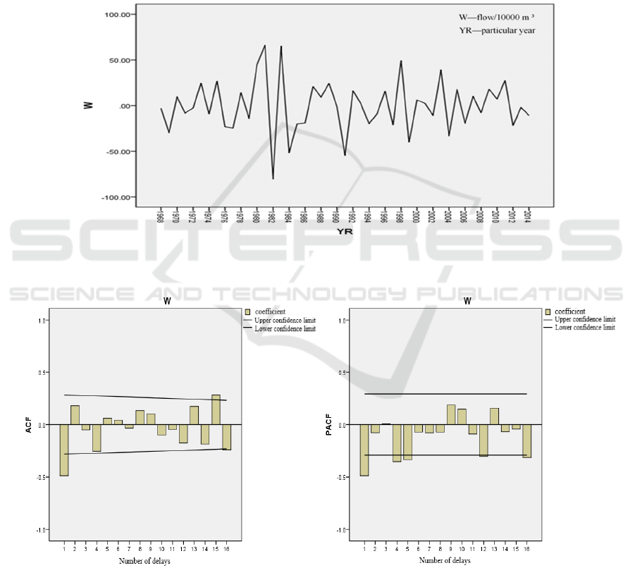
4.1 ARIMA Model Prediction

The annual runoff sequence of Yangxian Station in

the section of Han River in Shaanxi was selected for

ARIMA model prediction. Firstly, the stationarity

and pure randomness of the annual runoff sequence

of the Yangxian Station were analyzed by drawing

the time series diagram and autocorrelation diagram

of the annual runoff sequence. After judgment, the

station runoff time sequence is a non-stationary

sequence and a non-white noise sequence. Therefore,

it is necessary to carry out differential treatment to

the annual runoff series. In order to avoid the

phenomenon of over-differential, the annual runoff

sequence of Yangxian station is processed by

first-order difference (Figure 2), and the time series

graph after the difference and the autocorrelation

graph and partial autocorrelation graph are drawn, as

shown in Figure 3.

Figure 2: First order differential time sequence diagram of annual runoff sequence.

(a) Autocorrelation diagram (b) Partial autocorrelation diagram

Figure 3: First order differential autocorrelation and partial autocorrelation of runoff series.

It can be seen from (a) and (b) in Figure 3 that

the sequence has basically been a zero mean

stationary sequence after the first-order difference,

and the autocorrelation diagram is basically within

Research on Annual Runoff Forecast of Shaanxi Section of Hanjiang River Based on Multi-model

381

the confidence interval after the first-order lag time.

It can be judged that the autocorrelation function is a

first-order tail, and the partial autocorrelation

diagram decays rapidly to zero from the lag time of 2,

which can be preliminarily judged as truncated. In

order to ensure the accuracy of prediction, partial

autocorrelation is used as truncation and tailing, and

the model is established to select the optimal model.

Four models are determined through parameter trial

calculation: ARIMA (5,1,1), ARIMA (6,1,1),

ARIMA (5,1,0) and ARIMA (6,1,0). The four

models are tested and optimized. The statistics of

each model are shown in Table 1.

Table 1: Model parameter comparison.

Model

LB Statistics

BIC Value

Sequence Value DF Sig.b

ARIMA (5,1,1) 23.065 12 0.322 7.017

ARIMA (6,1,1) 22.120 11 0.169 7.103

ARIMA (5,1,0) 23.321 13 0.310 6.923

ARIMA (6,1,0) 23.809 12 0.242 7.022

It can be seen from Table 1 that the Q statistic P

value (Sig.b) of the residual sequences of the four

models are all greater than 0.05, indicating that the

residual sequences of the four models are all white

noise sequences. All four models are effective in

extracting the original sequence information

sufficiently. The optimal model is selected by the

BIC criterion. The smaller the BIC value, the better

the model. Therefore, the ARIMA (5,1,0) model with

the smallest BIC value is selected as the final model.

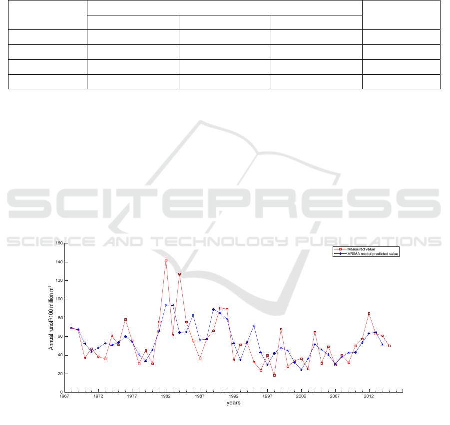
The model is used to predict the annual runoff

sequence of Yangxian Station, and the fitting curve

between the predicted value and the measured value

is shown in Figure 4. It can be seen that the predicted

value of ARIMA model does not fit well with the

measured value. Although the predicted sequence

can basically fit the trend of the measured sequence,

when the measured sequence rises and falls sharply,

the predicted sequence does not have the same

change law, and the predicted value also differs

greatly from the measured value, so the prediction

effect of ARIMA is poor.

Figure 4: Fitting diagram of the ARIMA Model forecasted and measured values.

4.2 Prediction of Mean-generating

Function

According to the basic principle of the mean

generating function model and formula (2), the mean

generating function is constructed based on the

annual runoff time series data of Yangxian station,

and the L-order mean generating matrix is obtained.

Then carry out periodic epitaxy according to formula

(3), and finally obtain the epitaxy matrix as follows:

WRE 2021 - The International Conference on Water Resource and Environment

382

53.67 53.67 53.67 53.67 53.67 53.67

56.62 50.73 56.62 50.73 56.62 50.73

52.06 58.93 69.56 52.06 69.56

































(12)

Thus, 24 predictors of the original annual runoff

series are obtained, conduct cross-correlation

analysis between each prediction factor and annual

runoff series, select the factors with good correlation

with the original series for multiple linear regression,

or consider all prediction factors for stepwise

regression. When modeling the mean generation

function, this paper considers the multiple regression

model, treats the selected factors equally, does not

distinguish the importance of each factor, and

ignores the independence of each factor. Therefore,

the model is established by stepwise regression of all

predictors, and then the 8 predictors most closely

related to the original sequence are selected

according to correlation analysis, and then the final

model is established by stepwise regression method

for prediction. First calculate the AIC value and BIC

value of the model, and the serial numbers of

predictors selected through correlation analysis are

15, 17, 18, 20, 21, 22, 23 and 24 respectively.

The final model is established by stepwise

regression method for prediction, and the parameters

and test statistics of the model are shown in Table 2.

It can be seen that only factor 22, factor 23, factor 17

and factor 15 are left after stepwise regression; The p

value (SIG) in F test is less than 0.05, indicating that

the overall linear regression of the model is

significant; The p value (SIG) in the t-test is also less

than 0.05, indicating that the regression coefficient

of the model passes the significance test, that is, the

remaining four factors (factors 22, 23, 17 and 15)

have a significant relationship with the annual runoff

series, and the model is effective. Therefore, the final

model is:

𝑦  25.773  0.481𝑥



 0.349𝑥



 0.319𝑥



 0.323𝑥



(13)

Table 2: MGF model correlation coefficient and test statistics.

Forecasting factors regression coefficient

F test t test

F Sig t Sig

constant

𝑏



-25.773

25.425 0

-2.989 0.005

Factor 22

𝑏



0.481 3.199 0.003

Factor 23

𝑏



0.349 2.134 0.039

Factor 17

𝑏



0.319 2.560 0.014

Factor 15

𝑏



0.323 2.047 0.047

The model is used to predict the annual runoff

series of Yangxian station, and the fitting curve

between the predicted value and the measured value

is obtained, as shown in Figure 5. It can be seen that

the prediction effect of the mean generation function

model is significantly better than the ARIMA model.

The prediction sequence of the mean generation

function model has the same change law as the

measured sequence. From 1967 to 1992, the

difference between the predicted value of the model

and the measured value is small, and the predicted

sequence and the measured sequence have a good

fitting effect, while from 1992 to 2007, the

difference between the predicted value and the

measured value becomes larger. The fitting degree

between the predicted sequence and the measured

sequence is general. Generally speaking, the

prediction effect of mean generation function model

is general.

Research on Annual Runoff Forecast of Shaanxi Section of Hanjiang River Based on Multi-model

383

Figure 5: Fitting diagram of MGF model forecast and measured values.

Figure 6: Fitting diagram of predicted values and measured values of GM (1, N) model.

4.3 Gray Dynamic Model Prediction

In this study, the annual runoff time series of

Yangxian station from 1967 to 2011 is taken as the

original data, that is, the prediction object. The

monthly average flow of this series from May to

October each year is taken as six prediction factor

series, and the GM (1, n) Grey dynamic prediction

model is established. Based on the established model,

the annual runoff of each year is predicted and tested

with the annual runoff from 2012 to 2014.

According to the basic principle of the model, the

1 - AGO series of each series can be calculated based

on the six series data of the monthly average flow.

These data are from May to October of the annual

runoff series of Yangxian Station. The calculation

results is the accumulation series, and then the

accumulation matrix B is obtained.The coefficient

vector a is obtained by using the least square method.

The parameters of the 𝐺𝑀  1,𝑁  model is

calculated as shown in Table 3.

Table 3: Annual runoff GM (1, N) model parameter calibration results.

Name of

parameter

Development

coefficient 𝑎

Driving coefficient

𝑏



𝑏



𝑏



𝑏



𝑏



𝑏



Constant Value 1.408426 0.004813 0.000698 0.000590 0.001919 0.000517 0.002650

In the above table, 𝑎 is the development

coefficient and the six driving coefficients are the

Grey action quantity of the model. Bring the model

parameters into formula (7) to obtain the time

WRE 2021 - The International Conference on Water Resource and Environment

384

response function of Grey dynamic model

𝐺𝑀 1,𝑛, and then restore according to formula (8)

to obtain the predicted value of annual runoff series

of Yangxian station. The fitting curve between the

predicted value and the measured value of the Grey

dynamic prediction model is shown in Figure 6. It

can be seen that the Grey dynamic model has a good

prediction effect on the annual runoff prediction of

Yangxian station. The prediction sequence has the

same change law as the measured sequence. The

predicted value of the model is close to the measured

value, and the predicted sequence has a good fit with

the measured sequence

4.4 DenseNet Model Building

This paper starts from the traffic data of Yangxian

Station on January 21, 1967, predicts the average

daily traffic of the previous nine days, takes the daily

traffic data of Yangxian Station on January 21, 1967

solstice on May 29, 2005 as the training data to train

the model, and the remaining data from 2006 to 2014

as the verification data. In order to train the model

effectively to improve the prediction accuracy and

make the model have better performance and

convergence speed, it is necessary to transform the

basic data in advance. The transformation formula is:

𝑧𝑎log



𝑥



𝑏 (where Z is the value after

transformation; 𝑎 is an arbitrary constant; 𝑥



is the

measured value, and b is generally 1). Then, the

predicted sequence obtained from the transformed

sequence is reduced according to the formula: 𝑥





/

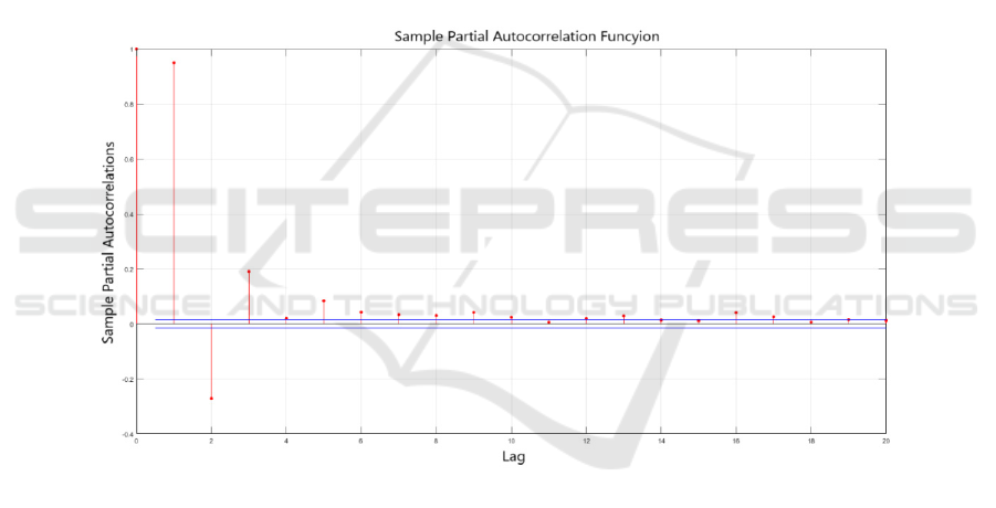
𝑏. In order to determine the model structure,

the partial autocorrelation diagram of the original

time series is also required, as shown in Figure 7.

Figure 7: Partial correlation diagram of original sequence.

As can be seen from Figure 7, the lag time is set

to 20, and after the lag time is 9, the partial

correlation coefficient basically remains stable and

oscillates in the upper and lower interval. Therefore,

the input layer of the model is set as nine neurons in

this paper. Through the trial algorithm, the number

of hidden layers is determined as three layers, and

each layer contains 30 neurons. The output layer is

set to the day forecast. Thus, the DenseNet model

structure was finally determined as 9-30-30-30-1.

After determining the model, first all the original

daily flow data are transformed, and then the training

set data are input into the model for training. Then,

the data of the validation set are used for verification,

and the prediction results of the training set and the

validation set are obtained. The predicted daily

average flow is restored, and the predicted annual

runoff of each year is finally accumulated and

calculated. The fitting curve between the predicted

value and the actual value of the DenseNet model is

shown in Figure 8. It can be seen that DenseNet

model has a good prediction effect on the annual

runoff prediction of Yangxian station. The prediction

sequence has the same change law of steep rise and

fall as the measured sequence. The difference

between the predicted value of the model and the

measured value is very small, and the predicted

sequence has a good fit with the measured sequence.

Research on Annual Runoff Forecast of Shaanxi Section of Hanjiang River Based on Multi-model

385

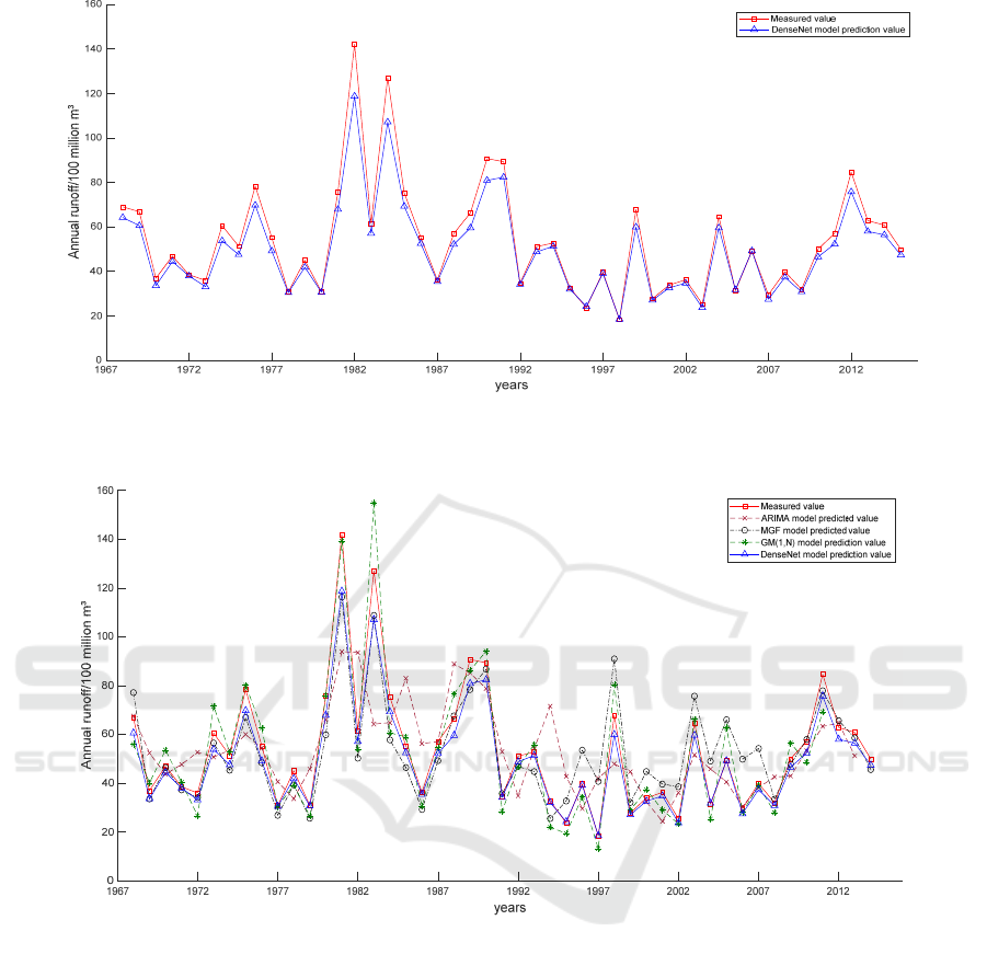
Figure 8: Fitting diagram of the predicted value of the DensetNet model and the measured.

Figure 9: Fitting Diagram of Predicted Values and Measured Values of Multiple Models.

5 COMPARATIVE ANALYSIS OF

MULTI-MODEL PREDICTION

RESULTS

The model is used to predict the annual runoff series.

The reliability of the model prediction result needs to

be tested after obtaining the prediction sequence

value. According to the Hydrological Prediction

specification, it is considered that the relative error of

one prediction is within plus or minus 20%, and the

qualified rate of prediction is calculated (Ministry of

Water Resources of the People's Republic of China,

2000), The average relative error MAPE, root mean

square error RMSE and certainty coefficient DC are

used to analyze the coincidence degree between the

predicted sequence and the measured sequence (Sun,

2012; Huang, 2015). The DC coefficient represents

the degree of coincidence between the predicted

sequence and the measured sequence. It and the

predicted qualified rate are maximized indicators, and

the greater its value, the better. MAPE and RMSE are

minimization type indicators. The smaller the value,

the better. The calculation results of the above four

indicators are shown in Table 4. The fitting diagram

between the predicted value of each model and the

measured value of annual runoff of Yangxian station

is shown in Figure 9.

WRE 2021 - The International Conference on Water Resource and Environment

386

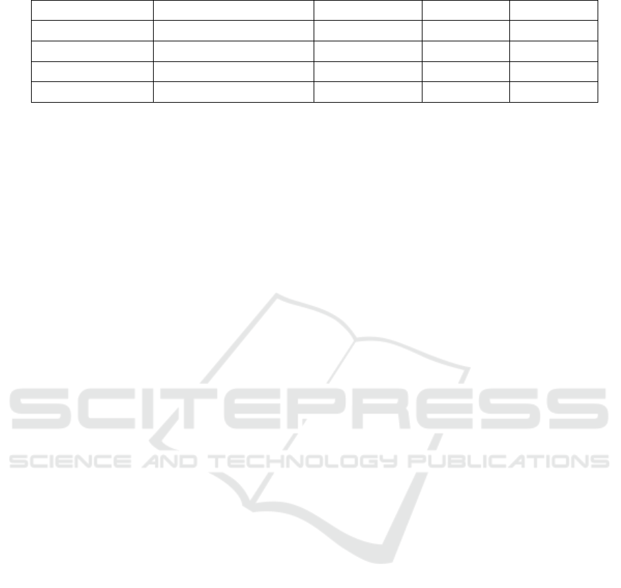
Table 4: Multi-model annual runoff forecast accuracy evaluation.

Model Qualification rate (%) MAPE (%) RMSE DC

ARIMA model 51.1 33.89 22.06 0.203

MGF model 72.9 19.47 13.40 0.801

Grey dynamic model 86.4 12.40 8.09 0.893

DenseNet model 100 6.39 6.18 0.937

According to the order of ARIMA model, MGF

model, 𝐺𝑀 1,𝑛 model and DenseNet model, it

can be seen from table 4 and Figure 9 that the

predicted qualified rate and DC coefficient are

getting larger and larger, the values of MAPE and

RMSE are getting smaller and smaller, and the

fitting degree between the predicted value series and

the measured value series is getting better and better.

Therefore, among the four models, ARIMA model

has the worst prediction effect. However, it can

basically show the trend of runoff series with large

error. The prediction effect of mean MGF model is

general. The prediction effect of Grey Dynamic

prediction model is better, and the prediction effect

of DenseNet model is the best. The prediction

qualified rate and DC coefficient of the prediction

results of DenseNet model are the largest, and

MAPE and RMSE are the smallest, showing obvious

advantages in all aspects. Therefore, for the annual

runoff prediction of Shaanxi section of Hanjiang

River, DenseNet model is the most suitable for the

annual runoff prediction of this area.

6 CONCLUSION

In this study, ARIMA, MGF model, Grey dynamic

prediction model and DenseNet model are used to

predict the annual runoff of Shaanxi section of

Hanjiang River. Through analysis and comparison,

the runoff prediction model most suitable for

Shaanxi section of Hanjiang River among the four

models is selected, which can improve the accuracy

of prediction results.

(1) Comprehensive comparative analysis of the

prediction results of the four models shows that

compared with ARIMA model, MGF model and

Grey Dynamic model, DenseNet model has the

highest prediction qualification rate, up to 100%, the

average relative error and root mean square are the

smallest, and the fitting effect is the best. It is most

suitable for the research of runoff prediction in

Shaanxi section of Hanjiang River.

(2) DenseNet model is the most suitable runoff

prediction model for the Shaanxi section of Hanjiang

River in this study. It is a runoff prediction model

based on neural network theory. In recent years,

some new theories have emerged in the field of

neural networks, such as Meshk (Huang, 2015)

theory. Densenet model can be used as a simple

template for creating neural network runoff

prediction model, and provide a reference for future

research.

(3) Appropriate runoff prediction models for

different regions can improve the accuracy and

rationality of runoff prediction, and provide

scientific and reasonable runoff prediction for

solving water problems such as water shortage,

water pollution, frequent flood disasters and urban

waterlogging. At the same time, it can also provide

basis for water conservancy departments to carry out

water regulation and rational allocation of water

resources, and provide guidance for reservoir

operation management and prevention Put forward

guidance on flood and drought relief, water

conservancy and power generation, agricultural

irrigation, etc.

ACKNOWLEDGMENTS

This research was funded by the Natural Science

Basic Research Program of Shaanxi Province (Grant

No. 2017JQ5076, 2019JLZ-16), Science and

Technology Program of Shaanxi Province (Grant

No.2019slkj-13, 2020slkj-16), the Scientific

Research Plan Program of Educational Department

Shaanxi Province (Grant No.17JK0558) and the

Program of Introducing Talents to Universities

(Grant Nos. 104-451016005 and 2016ZZKT-21).

The authors thank the editor for their comments and

suggestions.

REFERENCES

Cui, J. S., & Ye, L. (2009). Prediction analysis of annual

runoff of Harbin station based on stepwise regression

mean generation function model. Heilongjiang

Hydraulic Science and Technology, 37(04), 7-9.

Research on Annual Runoff Forecast of Shaanxi Section of Hanjiang River Based on Multi-model

387

Deng, J. L. (1982a). Control problems of grey systems.

Systems & Control Letters, 1(5), 288-294.

Deng, J. L. (1982b). The Grey Control System. Journal of

Huazhong University of Science and Technology

(Natural Science Edition), 3, 9-18.

Du, Y., & Ma, R. Y. (2018). Application of Different

Improved ARIMA Models in the Prediction of

Hydrological Time Series. Water Power, 44(04),

12-14,28.

Dutta, D., Welsh, W. D., & Vaze, J. (2012). A

Comparative Evaluation of Short-Term Streamflow

Forecasting Using Time Series Analysis and

Rainfall-Runoff Models in Water Source. Water

Resources Management, 26(15), 4397-4415.

Gu, H. Y. (2008). Study on the Forecasting of River

Runoff. Northeast Forestry University.

Huang, Q. L. (2015). Study on runoff prediction model of

Jinghe River Basin. Northwest A&F University.

Hsu, K. L., Gupta, H. V., & Sorooshian, S. (1995).

Artifical Neural Network Modeling of the

Rainfall-Runoff Process. Water Resources Research,

31(31), 2517-2530.

Labat, D., Godderis, Y., & Probst, J. L. (2004). Evidence

for global runoff increase related to climate warming.

Advances in Water Resources, 27(6), 631-642.

Lei, S. P., Ruan, B. Q., & Xie, J. C. (2003). Function of

Water Resource on Human Civilization Innovation

Mechanism. Journal of Northwest A&F University

(Social Science Edition), 3(6), 61-65.

Li, J., Wang, L., & Ma, G. W. (2008). Application of Least

Squares Support Vector Machines in Runoff Forecast.

China Rural Water and Hydropower, 5, 8-10.

Liang, H., Huang, S. Z., Meng, E. H., & Huang, Q. (2020).

Runoff prediction based on multiple hybrid models.

Journal of Hydraulic Engineering, 51(01), 112-125.

Liu, D. L. (2011). Study on ARIMA model prediction of

annual precipitation and soil and water conservation

in Zhengzhou. Research of Soil and Water

Conservation, 18(6), 249-251.

Liu, S. F., & Yang, Y. J. (2015). Advance in Grey System

Research (2004-2014). Journal of Nanjing University

of Aeronautics & Astronautics, 47(1), 1-18.

Liu, X. A., Wang, J. W., & Wang, H. W. (2006). Wavelet

Analysis-based ARIMA Method for Monthly Runoff.

Forecast Hydroprower and Pumped Storage, 4(04),

77-80.

Ministry of Water Resources of the People's Republic of

China. (2000). SL 250-2000 code for hydrological

information forecast. Beijing: China water resources

and Hydropower Press.

Schreider, S. Y., Jakeman, A. J., & Dyer, B. G. (1997). A

combined deterministic and self-adaptive

stochasticalgorithm for streamflow forecasting with

application to catchments of the Upper Murray Basin,

Australia. Environmental Modelling & Software,

12(1), 93-104.

Sun, H. Z. (2012). A Variety of Combination Forecasting

Method and Comparing of Medium and Long-term

Stream-flow. Northwest A&F University.

Sun, M., Kong, X. C., & Geng, W. H. (2013). Time series

analysis of monthly precipitation in Shandong

Province Based on ARIMA model. Journal of

Ludong University (Natural Science Edition), 29(3),

244-249.

Wei, F. Y., & Cao, H. X. (1990). The mathematical model

of long - term forecasting and its application. Beijing:

China Meteorological Press.

Xia, J., & Ye, S. Z. (1995). Grey System Approach

Applied to Flood and Runoff Forecasting. Water

Resources and Power, 3, 197-205.

Xiong, B. X., & Chen, F. (1987). Hydrological

Characteristics of the Upper Hanjiang River in

Shaanxi Province. Power System and Clean Energy,

1, 9-16.

Xu, J. X., Li, Z. Q., & Zhang, F. (2005). Application and

Research of Grey System Theory in Surface Runoff

Forecast. Journal of North China University of Water

Resources and Electric Power (Natural Science

Edition), 26(3), 1-3.

Zeng, W. B., & Lin, L. J. (2010). Prediction of Monthly

Runoff in the Upper Reaches of Qingyi River Based

on GM (1,1) Model Shaanxi. Journal of Agricultural

Sciences, 56(05), 92-94.

Zheng, S. W., & Shi, B. (2010). Study on annual runoff

prediction based on improved grey system theory.

Yellow River, 32(02), 40-41.

WRE 2021 - The International Conference on Water Resource and Environment

388