Experimental Study on the Turbulent Flow Field inside Hydrocyclone

with Particle Image Velocimetry

Xu Duan

TSI Instrument (Beijing) Co., Ltd, Beijing, China

Keywords: Particle Image Velocimetry (PIV), Turbulent flow field, Axial velocity, Radial velocity, Secondary vortexes

Abstract: The hydrocyclone separation is highly related to its flow field. The investigation of the turbulent flow

characteristics helps the optimization of the hydrocyclone structure design. In this article, the turbulent flow

field in a 50mm hydrocyclone was investigated with Particle Image Velocimetry. The cylinder section and

part of the cone section are measured simultaneously. Both the axial and radial velocity components peak in

the central area of the hydrocyclone. But for radial velocity, it varies between inward and outward from top

to bottom, not exclusively inward in the cone section. The secondary vortexes exist in the transition area of

inner spiral flow and outer spiral flow, where higher vorticity is located. Turbulent intensity and Reynolds

shear stress is calculated from the two velocity components with time series. It has been made clear that the

central area is where the turbulence is strongest. And the maximum radial turbulence intensity exists in the

vicinity of vortex finder tip, while maximum axial turbulence intensity exists in the lower cone section with

transition of flow. Results show the averaged velocity field is smoother and more convenient for

comprehending while the instantaneous velocity field is less distorted by the averaging process.

1 INTRODUCTION

Hydrocyclone has been widely used for its

simplicity in manufacturing and efficiency in

long-term running. But the flow field, which

explains how the separation is working, is more

complicated to make clear.

The difficulties should be attributed to the

turbulent and three-dimensional characteristics.

Previous works mostly relied on Laser Doppler

Velocimetry (LDV) or Phase Doppler Particle

Analyzer (PDPA) measurements (Bergstrom &

Vomhoff, 2007), which only measured the two or

three components of velocity in a single point. Since

the measurement of points is not conducted

simultaneously, it becomes problematic to discuss

the instantaneous velocity profile. The PDPA results

were sampled by hundreds or even thousands of

single-point data of velocity components in one

interval of time. Most previous works on

hydrocyclonic flow field measurements with PDPA

were displaying averaged velocity profile (Yang et

al., 2011). Of course, some researchers did present

some turbulence information, such as RMS value

(Zhang et al., 2009). But data is restricted in a

certain vertical position and it’s impossible to have

an overall view on the hydrocyclone flow field.

Another problem is the measurement of radial

velocity. The ordinary configuration of PDPA is

only able to measure the tangential and axial

velocity. Even though the 3D PDPA has been

developed recently, the relatively lower value of

radial velocity makes it even more difficult to get

convincing conclusion.

Although Particle Image Velocimetry (PIV) is a

common and mature measurement method, its

application in hydrocyclone measurement is rare. In

fact, PIV is very suitable to measure the velocity

field inside hydrocyclone, especially the turbulent

feature and the specific features such as secondary

vortexes. Marins et al. (2010) measured the velocity

field in a hydrocyclone with both LDA (similar to

PDPA) and PIV, but the area of interest for PIV is in

a 1° cone near underflow, where the hydrocyclone

wall is thin enough. And he discussed the turbulence

data based on LDA measurement. Lim et al. (2010)

measured both cylindrical section and cone section

with PIV, but he used it mainly for the validation of

CFD result and didn’t draw impressive conclusions.

Little literature focused on the hydrocyclone flow

field measurement with PIV, but some research on

gas cyclone measurement is inspiring. Zheng and

Duan, X.

Experimental Study on the Turbulent Flow Field inside Hydrocyclone with Particle Image Velocimetry.

In Proceedings of the 7th International Conference on Water Resource and Environment (WRE 2021), pages 219-225

ISBN: 978-989-758-560-9; ISSN: 1755-1315

219

Wong made a comprehensive studied on a gas

cyclone (Zheng et al., 2006; Wong et al., 2007). He

divided the cyclone into three sections and measured

separately. The problem is that the sections were not

connected and not measured simultaneously. This

means the loss of some specific features of

secondary vortexes throughout the cross-section.

In this article, the flow field inside an optical

glass 50mm hydrocyclone was measured with

Particle Image Velocimetry (PIV). The

instantaneous velocity profile and vorticity profile is

presented and made comparison with their average

counterparts. The other turbulent information, such

as turbulent intensity and Reynolds shear stress are

also discussed.

2 EXPERIMENTAL

2.1 Hydrocyclone Model

The geometry of Φ50mm hydrocyclone for PIV test

is shown in Figure 1 and the detailed parameter is in

table 1. This type of hydrocyclone in is mainly

designed for solid-liquid separation, for example, the

Methanel to Olefin (MTO) quench water treatment.

Optical grade fused quartz (JGS2) was chosen as the

material of the cyclone body, for considering its

good UV and visible transmission. The optical grade

fused quartz is relatively low for refractive index,

which make it suitable for image measurement

methods.

Figure 1: The geometry of hydrocyclone.

Table 1: Dimensions of the hydrocylone.

D/mm 50

L1/D 1.48

L2/D 8.78

do/D 0.24

Do/D 0.68

du/D 0.08

d/mm 8

h/mm 12

2.2 Experimental Setup

2.2.1 Experimental Procedure

As is shown in Figure 2, water was pumped from a

50L tank to a buffer vessel for a smoother pressure

profile, and then into the hydrocyclone through the

rectangular tangential inlet. Both the overflow and

the underflow went back to the tank to complete a

circulation of the feed material. Hollow glass

microspheres were seeded to trace the fluid flow.

The medium size of the tracer particles is around

10μm, while their particle density is about

1100g/cm3. Three pressure gauges were fixed on all

the inlet and outlets to determine the feed pressure

and control the split ratio. To eliminate the distortion

created by the phenomenon of refraction, we

introduced an index matching method for the

acquisition of images with improved quality. The

hydrocyclone is put inside a rectangular PMMA box

and filled with water inside and outside the

hydrocyclone. Thus, the distortion of image was

minimized for a better result.

Figure 2: Experimental setup.

WRE 2021 - The International Conference on Water Resource and Environment

220

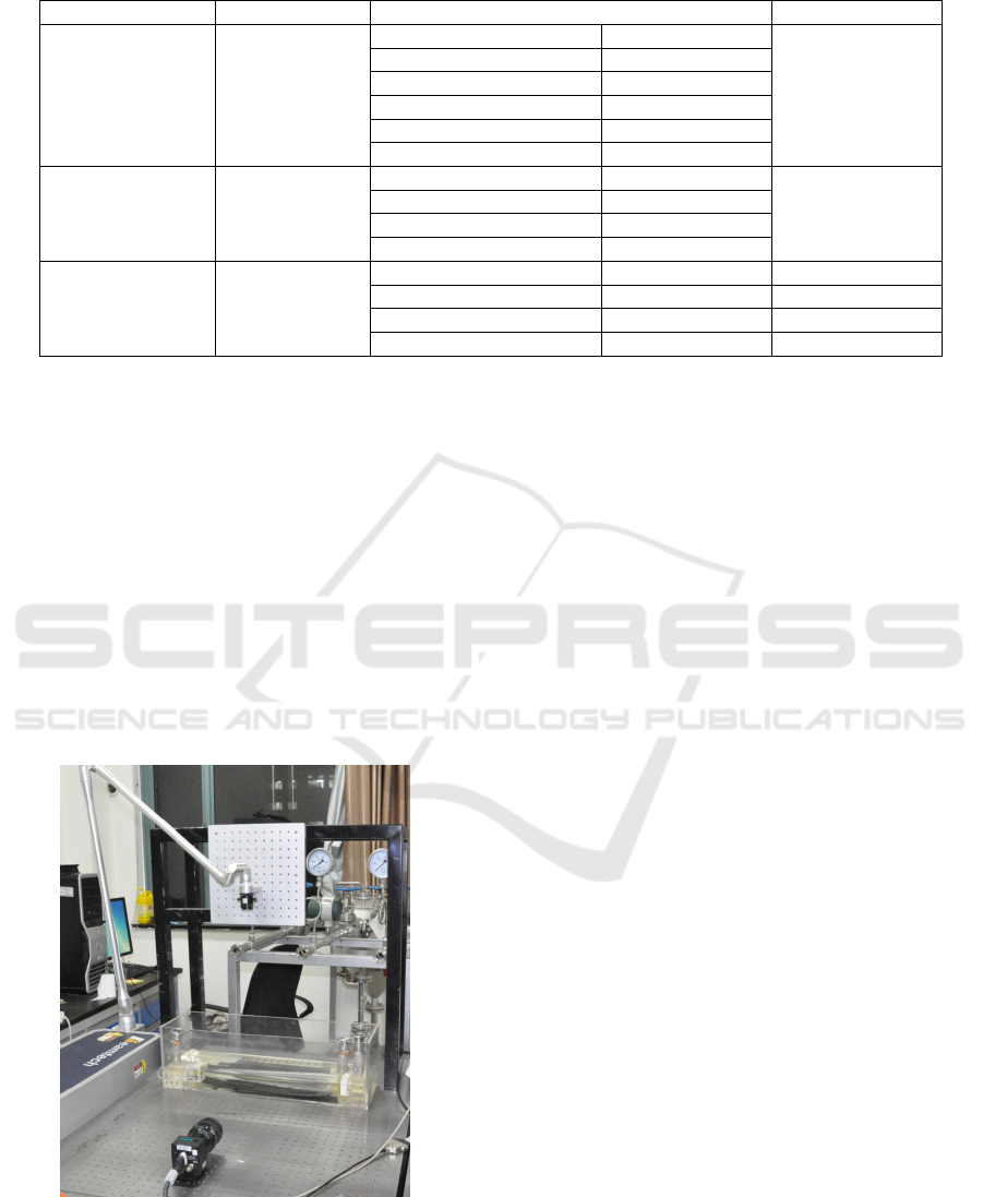
Table 2: Instrumentation.

Setup Model Parameter of Apparatus Manufacturers

Nd:YAG Laser Vlite-500

Wavelength 532 n

Beamtech

Energ

500 mJ/Pulse

Pulse Duration 6-8 ns

etition Rate 15 Hz

Beam Size 8 m

Timing Jitte

2 ns

Synchronizer 610035

Dela

0-1000s

TSI

Pulsewidth 10ns-1000s

Resolution 1ns

Jitte

<400

CCD Camera 630159

Pixel Resolution 400,82,672

ixels TSI

Frame Rate 15 fps

Frame Straddling Time 200ns

Camera Lens 60m

Nikon

2.2.2 Instruments for Measurement

The particle image is captured with a TSI 630159

CCD system. To get images with better quality, a

Nikon 60mm micro-lens is mounted to the TSI

camera. The light sheet is created with the

combination of cylindrical lens and spherical lens.

The two lenses are mounted in the front of laser

emitter of the light arm, which guides the light from

the laser device. The detailed components of

instrumentation are shown in Table 2. Figure 3 show

the measurement instruments of hydrocyclone for

PIV test.

Figure 3: The measurement instruments.

3 RESULTS AND DISCUSSION

3.1 The Axial Velocity Profile

In this experiment, the flow inside hydrocyclone is

operated to a quasi-stable state with no air-core. A

set of two particle images of the central plane

orthogonal to the inlet are captured instantaneously.

The capture interval Δt between the two images of

one straddle is set to 100μs and the exposure time is

300μs. The PIV measurement of flow field inside

hydrocyclone is repeated by 200 times to obtain an

averaged velocity profile.

Figure 4 shows the axial velocity with the Locus

of Zero Vertical Velocity (LZVV) with the inlet

pressure at 50kpa, 100kpa and 150kpa. It can be seen

that the upward axial velocity magnitude peaks in

the central area. The downward axial velocity peaks

in the vicinity of the hydrocyclone wall. The axial

velocity in the area around the LZVV is very slight

in value, where the primary flow will stay longer

inside the hydrocyclone before discharged from the

underflow orifice or overflow pipe. The locus

divides the hydrocylone into two areas: one

promoting the separation process (with downward

axial velcoity) and the other detrimental. From the

three axial velocity contour maps under different

inlet pressure, the LZVV are in the same shape for

similar split ratio of the hydrocyclone. And the locus

is located around 1/6 radius of the cylinder section

away from the hydrocyclone wall.

Experimental Study on the Turbulent Flow Field inside Hydrocyclone with Particle Image Velocimetry

221

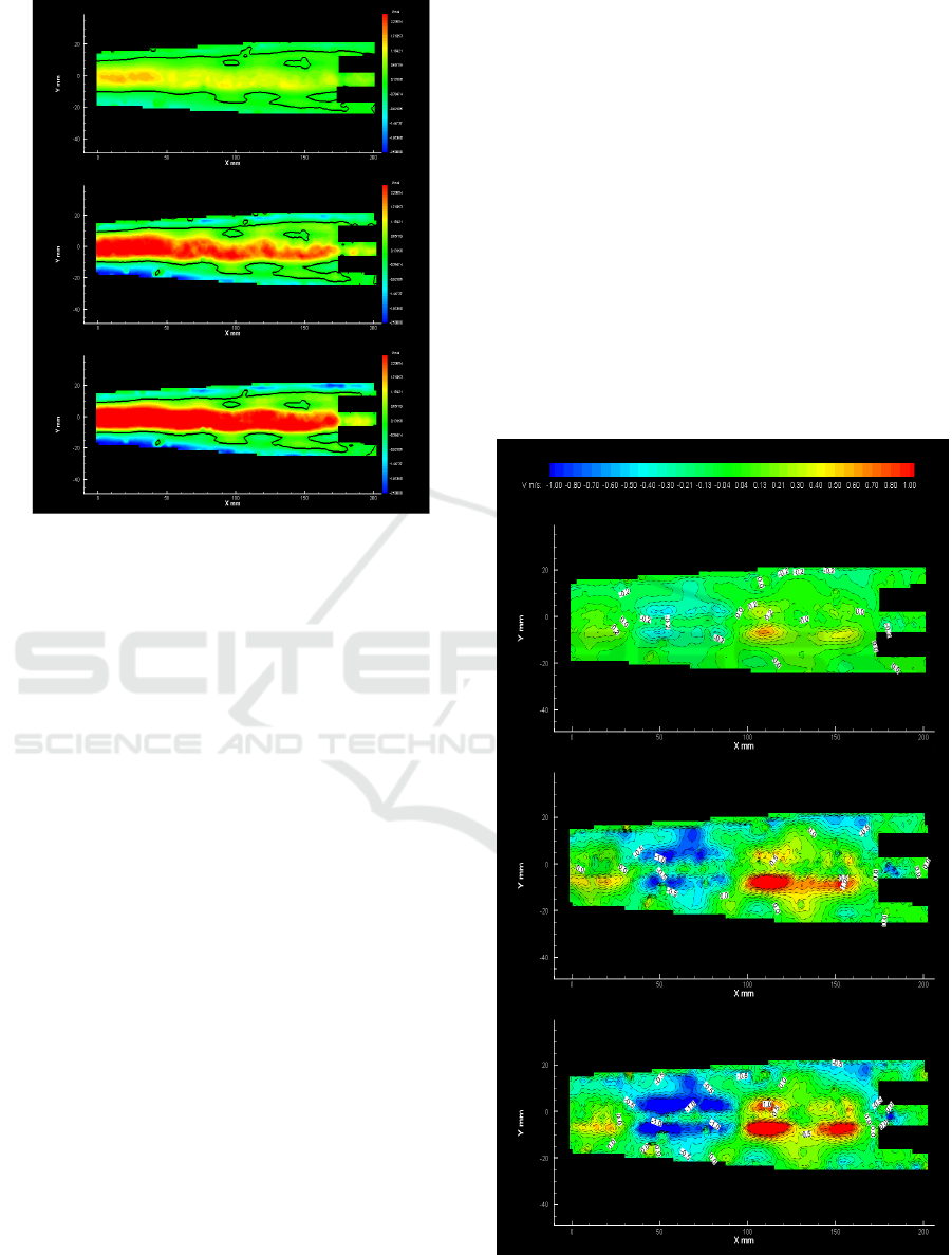
Figure 4: The axial velocity contour. contoury

(LZVV)tantaneous vector map of hydrocyclone flow filed.

3.2 The Radial Velocity Profile

Figure 5 shows the radial velocity profile with the

inlet pressure at 50kpa, 100kpa and 150kpa. The

radial velocity is asymmetric even in absolute value.

The asymmetric in absolute value may be attributed

to the single injection of flow. It’s obvious that the

radial velocity peaks in the area very close to the

axis. The peak radial velocity is around 20% of the

axial flow. Although the hydrocyclone is operated

without an air-core, there still exist some upward

flows in the central area with little radial movement.

Another feature of the radial velocity profile is its

variation along axis. It is of great difference from

axial velocity component (or tangential velocity

component) that the radial velocity varies sharply

between outward direction and inward direction. But

most former researchers reported inward velocity in

the cone section, depending on their PDPA

measurements (Bergstrom & Vomhoff, 2007). And

Luo et al. (1989) concluded it with an equation

shown as following:

rc

It was the single-point feature of measurements

with PDPA that resulted in this misunderstanding.

The radial velocity is more complicated than it was

previously deemed. It was clear with PIV

measurements hat the radial velocity is inward in the

upper cone section in only one half of the

hydrocyclone. As a matter of fact, except for the

limited area near hydrocyclone wall, the inward

radial velocity will be replaced by outward radial

velocity in the lower cone section. And the radial

velocity profile is just the opposite in the other side

of the axis. As to the inward radial velocity profile

along axial direction in cone section, it will increase

to the maximum and then decrease to zero and

finally replaced by outward velocity. Thus, the radial

velocity equation should be modified to satisfy this

situation. We can keep the assumption that the radial

velocity followed the similar regulation of tangential

velocity in the inward region. But for the outward

region, the constant -c should be positive. What’s

more, it is obvious that the constant m and C should

be changing along axial direction.

Figure 5: The radial velocity contour.

WRE 2021 - The International Conference on Water Resource and Environment

222

3.3 The Two-dimensional Velocity and

Vorticity Profile

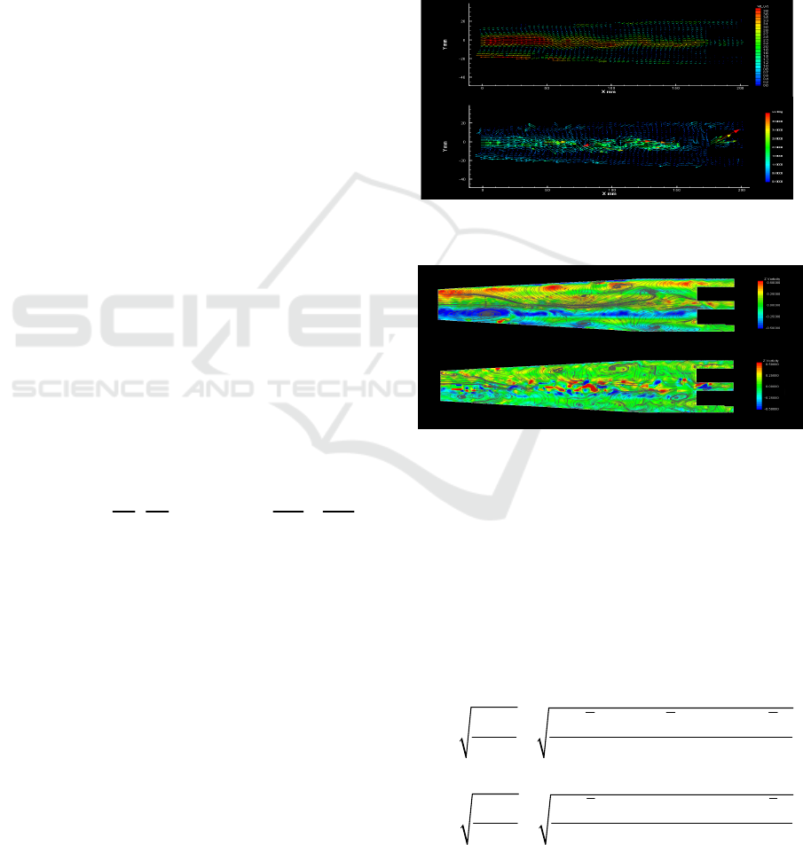
The averaged two-dimensional two-component

(2D2C) velocity profile is shown in Figure 6(a).

For the three visualizations of hydrocyclonic

flow field with the inlet pressure at 50kpa, 100kpa

and 150kpa, the vector maps are very similar for the

structure, but the velocity magnitude increases with

increasing inlet pressure. The peak values of velocity

magnitude of all the three visualizations are located

in the central axis of the hydrocyclone. The velocity

vectors are pointed downward near wall and upward

near the axis. This information gives a general idea

for the averaged two-dimensional two-component

(2D2C) velocity profile.

Another significance of the 2D2C velocity

profile is the identification of secondary vortexes.

Figure 7(a) shows the diagram of streamlines

imposed on the vorticity contour. It can be seen that

the vortexes are distributed between the central axis.

The vortexes are in the same rotation sense when

located in the same half, denoting similar formation

mechanism. The secondary vortexes are long

recognized as the “mantle” which is detrimental to

particle transportation from axis to wall. Although

the influence of secondary vortexes is not clear so

far, it’s worth paying attention to its characteristics.

The vorticity distribution profile also denotes the

rotation sense. The Z vorticity



that is presented in

Figure 6 represents the degree of local fluid rotation

and valuable for the determination of the vortex

characteristic and turbulence. The Z vorticity



calculated with the following equation:

(,)(,)

vvv

yxy







    

  



The relatively higher vorticity is located in the

transition area of inner spiral flow and outer spiral

flow. The location is also where secondary vortexes

exist, mainly owing to the sharp transition of the

primary flow. The local rotation of fluid would

influence a lot to the particle behavior. If consider a

group of particle transporting from axis to wall and

experiencing a secondary vortex, the particles will

inevitable rotate by themselves and the mass transfer

process will be enhanced.

In comparison with the instantaneous velocity

vector map in Figure 6(b), the averaged velocity

profile is smoother and more convenient for

comprehending. But in another hand, the

instantaneous velocity profile is not distorted by the

averaging process. The instantaneous streamline

superimposed on the vorticity contour map (with the

inlet pressure at 100kpa) is presented in Figure 7(b).

We found some extra secondary vortexes in the

instantaneous map. This indicates that in the

turbulent flow field inside hydrocyclone, the

large-scale secondary vortexes are not able to keep

always stable, and they will break up to form several

smaller scale vortexes. The comparison of the two

streamline diagrams also demonstrates that the

averaging process will eliminate some detailed

structures in the flow field.

Figure 6: Averaged and instantaneous vector map of

hydrocyclone velocity field.

Figure 7: Typical streamline superimposed on the vorticity

distribution contour map.

3.4 The Turbulent Intensity

Figure 8 and Figure 9 shows the standard deviation

of axial velocity and radial velocity, respectively.

The standard deviation is calculated from the 200

visualizations of the velocity field inside

hydrocyclone. The standard deviation σ for axial

velocity and radial velocity are defined by the

following equations:

22 2

-+ -+...+ -

uu uu uu







（

）（）（）

i=1,2,…,n

22 2

- + - +...+ -

vv v v vv







（

）（）（）

i=1,2,…,n

Experimental Study on the Turbulent Flow Field inside Hydrocyclone with Particle Image Velocimetry

223

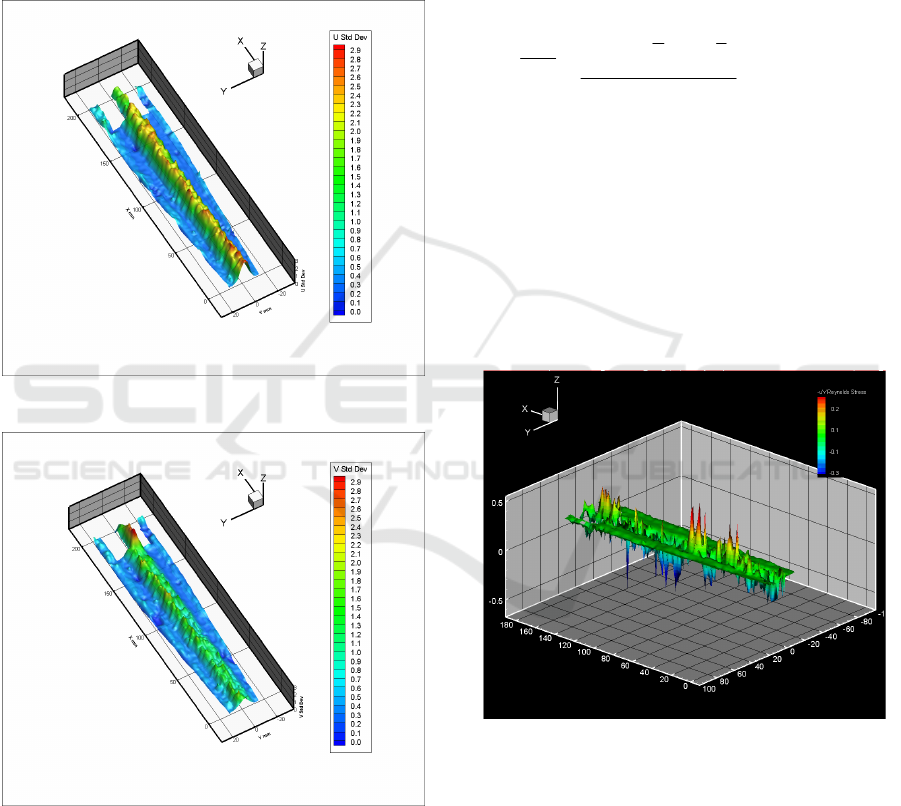
The standard deviation σ is also called the

turbulent intensity, representing the degree of

velocity variation in the turbulent flow. Its square is

the same with non-normalized Reynolds normal

stress. In Figure 7, the standard deviation of axial

velocity is rather slight at the quasi-free vortex area.

The turbulence there is not so strong in comparison

to that in the forced vortex area. And the relatively

higher axial velocity in the forced vortex area also

contributes a lot to this phenomenon.

Figure 8: The standard deviation of axial velocity.

Figure 9: The standard deviation of radial velocity.

As is shown in Figure 8, the standard deviation

of axial velocity is also higher in the forced vortex

area. But it peaks in the vicinity of the vortex finder,

while the standard deviation of axial velocity peaks

in the lower part of the cone section. Experimental

results show the radial velocity in the vicinity of the

vortex finder is not so high, which indicates the

turbulence there is rather strong. This reminds us to

modify the vortex finder shape or size to reduce the

turbulence and minimize the bad influence of

back-mixing in some classification process.

3.5 The Reynolds Shear Stress

The Reynolds shear stress is the index for turbulent

fluctuations in fluid momentum. It is obtained from

the averaging process over the Navier-Stokes

equations and defined by the following equation:

"''

(-)(-)

ij i j

uuv v







i=1,2,…,n;

j=1,2,…,n

Figure 10 shows the Reynolds shear stress in the

surface. It is found that the much higher Reynolds

shear stresses are produced in the central area. The

lower values are found in the vicinity of

hydrocyclone wall. It demonstrates again the central

area of the hydrocyclone is where the turbulence

concentrates. The data of Reynolds stress could also

serve as the reference for model validation and

modification.



Figure 10: The Reynolds stress.

4 CONCLUSIONS

The turbulent flow field in a 50mm hydrocyclone

was investigated with Particle Image Velocimetry.

200 visualizations were averaged and analyzed.

Results show the averaged velocity field is smoother

and more convenient for comprehending while the

instantaneous velocity field is less distorted by the

averaging process. Both the axial and radial velocity

WRE 2021 - The International Conference on Water Resource and Environment

224



components peak in the central area of the

hydrocyclone. But for radial velocity, it varies

between inward and outward from top to bottom, not

exclusively inward in the cone section. For the

secondary flow pattern, it is found that the secondary

vortexes exist in the transition area of inner spiral

flow and outer spiral flow, where higher vorticity is

located. Turbulent intensity and Reynolds shear

stress is also calculated from the two velocity

components with time series. It is made clear that the

central area is where the turbulence is strongest. And

the maximum radial turbulence intensity exists in the

vicinity of vortex finder tip, while maximum axial

turbulence intensity exists in the lower cone section

with transition of flow.

REFERENCES

Bergstrom, J., & Vomhoff, H., (2007). Experimental

hydrocyclone flow field studies. Separation and

Purification Technology, 53, 8-20.

Lim, E. W. C., Chen, Y. R., Wang, C. H., & Wu, R. M.,

(2010). Experimental and computational studies of

multiphase hydrodynamics in a hydrocyclone

separator system. Chemical Engineering Science, 65,

6415-6424.

Luo, Q., Deng, C., Xu, J. R. Yu, L. X., & Xiong, G. G.,

(1989). Comparison of the performance of

water-sealed and commercial hydrocyclones.

International Journal of Mineral Processing, 25,

297-310.

Marins, L. P. M., Duarte, D. G., Loureiro, J. B. R., Moraes,

C. A. C., & Freire, A. P. S., (2010). LDA and PIV

characterization of the flow in a hydrocyclone without

an air-core. Journal of Petroleum Science and

Engineering, 70, 168-176.

Wong, W. O., Wang, X. W., & Zhou, Y., (2007). Turbulent

flow structure in a cylinder-on-cone cyclone. Journal

of Fluids Engineering, 129, 1179-1185.

Yang, Q., Wang, H. L., Wang, J. G., Li, Z. M., & Liu, Y.,

(2011). The coordinated relationship between vortex

finder parameters and performance of hydrocyclones

for separating light dispersed phase. Separation and

Purification Technology, 79, 310-320.

Zhang, Y. H., Liu, Y., Qian, P., & Wang, H. L., (2009).

Experimental Investigation of a Minihydrocyclone.

Chemical Engineering & Technology, 32, 1274-1279.

Zheng, Y., Liu, Z. L., Jiao, J. Y., Zhang, Q. K., & Jia, L. F.,

2006. Investigation of turbulence characteristics in a

gas cyclone by stereoscopic PIV. Aiche Journal, 52,

4150-4160.

Experimental Study on the Turbulent Flow Field inside Hydrocyclone with Particle Image Velocimetry

225