Community and Distribution of Living Coccolithophores in the

Yellow Sea and East China Sea

Jian Zhang

, Yi Yang

1,*

, Zhaoyang Liu

, Youquan Zhang

and Xueding Li

National Marine Data and Information Service,Tianjin, 300171, China

Fu Jian Marine Forecasts, Fujian, 350003, China

Keywords: Living coccolithophores, Community and distribution, Yellow Sea and East China Sea, Summer and Winter

Abstract: Based on the investigation and study on the community and distribution of Living coccolithophores (LC) in

the Yellow Sea and East China Sea in summer and winter 2016. In summer, 21 species of LC were found in

the survey area, and their dominant species were E. huxleyi, G. oceanica, U. tenuis and F. profunda. The cell

abundance ranged from 0.023 to 1.762 × 104 cells/L, with an average of 0.284 × 104 cells/L. In winter, 20

species of LC were found in the survey area, and their dominant species were E. huxleyi, G. oceanica, F.

profunda and U. tenuis. The abundance of LC ranged from 0.012 to 3.535×104 cells/L, with an average of

0.384×104 cells/L. This thesis investigated and analyzed the LC community and distribution in two seasons

(summer and winter) of the Yellow Sea and East China Sea, which enriched the LC studies in the coastal

seas of China and also provided the basic data for understanding carbon cycle and carbon flux in China Sea

waters.

1 INTRODUCTION

Living coccolithophores (LC) refer to those who live

in the sea today, with calcium carbonate shells at

certain stages of life history, and play an important

role in the marine ecosystem (Billard & Inouye,

2004). LC take a great part in the marine carbon cycle

process, and as one of the most important producers

in the marine ecosystem. With its unique carbonate

counter pump and organic carbon pump, LC take a

great part in the ocean’s carbon cycle (Sun, 2007). So

far, the community and distribution (especially

vertical distribution) of LC is still not clear in China

Sea. Based on the investigations of the communities

and distribution of LC in the Yellow Sea and East

China Sea in summer (20th July to 1st September)

and winter (23th December to 5th February) in 2016,

we made a report about the LC species composition,

cell abundance, dominant species, horizontal

distribution, vertical distribution, diversity index and

evenness index from upper body water (0 ~ 200m).

Lacking of internationally harmonized method for

quantitative sampling and sample analysis, This

study applied the polarizing microscope method

(Bollmann et al., 2002) which is widely recognized

internationally and can truly reflect quantitative

information, and its description and analysis was

made in order to provide reliable information on the

basis of the study of LC community about

distribution, and for China's coastal waters follow-up

studies of carbon fluxes, coccolithophores

calcification and its response to global climate

change and other support.

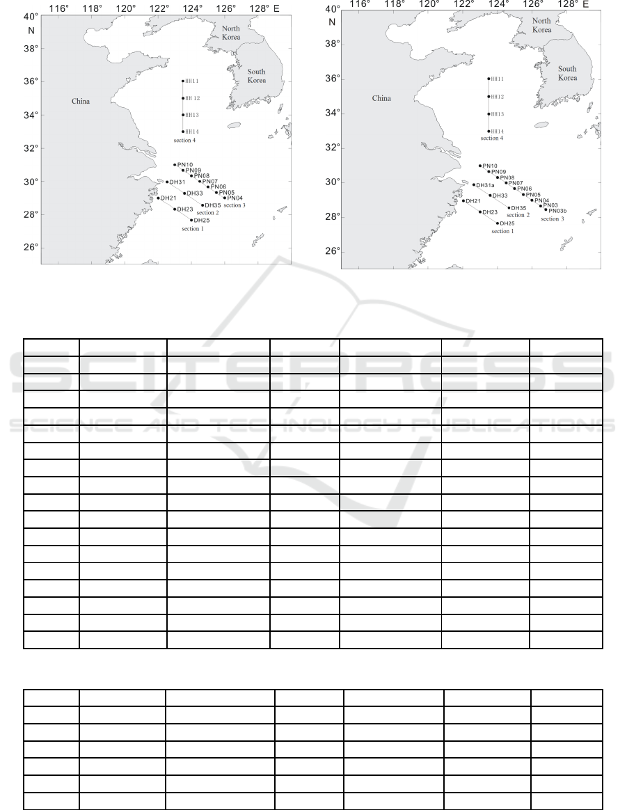
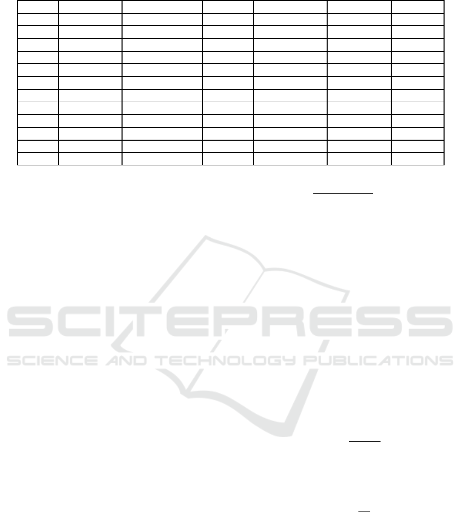
2 SURVEY AREAS AND

RESEARCH METHODS

2.1 The Survey Areas

This study was based on China's coastal waters

investigation. Respectively, in summer (July 20 to

September 1) and winter (December 23 to February

5th) of China Sea waters (27.00 ° ~ 36.50 ° N, 121.50

° ~ 127.00 ° E), including water chemistry, chemical

and biological, with a comprehensive field

investigation nested two quarters of the month. In

summer and winter, 17 and 19 survey sampling

stations were set up in the survey areas (Figure 1,

Figure 2). Meanwhile, there were four sections

(section 1, section 2, section 3, section 4) located in

the survey area. The information of sampling stations

was listed in Table 1 and Table 2. LC samples were

collected from the surface (~ 2 m) below the natural

Zhang, J., Yang, Y., Liu, Z., Zhang, Y. and Li, X.

Community and Distribution of Living Coccolithophores in the Yellow Sea and East China Sea.

In Proceedings of the 7th International Conference on Water Resource and Environment (WRE 2021), pages 151-163

ISBN: 978-989-758-560-9; ISSN: 1755-1315

151

water by using CTD, and then poured into the sea to

get a 1L polyethylene bottle, immediately adding the

right amount of weakly alkaline solution of formalin,

making the concentration of formaldehyde in the

sample of 1% to 2% (Sun, 2007). Temperature and

salinity were determined by the ship's CTD.

Figure 1: 2016 summer survey stations bitmap. Figure 2: 2016 winter survey stations bitmap.

Table 1: Summer survey stations of 2016.

Stations Regions Date Time Longitude Latitude Depth

DH21 ECS 2016-8-20 8:29 122.0113

28.9926

DH23 ECS 2016-8-20 15:41 123.0002

28.3306

DH25 ECS 2016-8-20 23:40 124.0016

27.6627

DH35 ECS 2016-8-22 3:55 124.6662

28.5573

DH33 ECS 2016-8-22 11:07 123.5851

29.2843

DH31 ECS 2016-8-22 20:00 122.5414

29.9651

PN10 ECS 2016-8-24 17:57 123.0006

31.0004

PN09 ECS 2016-8-24 21:38 123.4950

30.6715

PN08 ECS 2016-8-25 2:19 124.0011

30.3325

PN07 ECS 2016-8-25 6:10 124.4998

29.9981

PN06 ECS 2016-8-25 10:41 124.9993

29.6716

PN05 ECS 2016-8-25 15:04 125.4994

29.3309

PN04 ECS 2016-8-25 20:25 125.9969

29.0026

117

HH14 YS 2016-8-29 14:06 123.4990

32.9972

37.4

HH13 YS 2016-8-29 23:30 123.5035

34.0009

HH12 YS 2016-8-30 9:00 123.5012

34.9981

77.8

HH11 YS 2016-8-31 12:23 123.4938

36.0400

Table 2: Winter survey stations of 2016.

Stations Regions Date Time Longitude Latitude Depth

PN03b ECS 2016-12-26 16:30 126.8008 28.4618 209

PN03 ECS 2016-12-26 19:59 126.5000 28.6667 134

PN04 ECS 2016-12-27 0:58 126.0000 29.0000 118

PN05 ECS 2016-12-27 5:11 125.5067 29.3256 94

PN06 ECS 2016-12-27 9:55 125.0000 29.6710 83

PN07 ECS 2016-12-27 13:28 124.5000 30.0000 68

WRE 2021 - The International Conference on Water Resource and Environment

152

PN08 ECS 2016-12-28 8:30 124.0028 30.3266 50

PN09 ECS 2016-12-28 11:50 123.5003 30.6683 58

PN10 ECS 2016-12-28 16:29 123.0000 31.0000 49

DH31a ECS 2016-12-29 5:06 122.6394 29.8914 36

DH33 ECS 2016-12-29 12:16 123.5792 29.2799 69

DH35 ECS 2016-12-29 19:42 124.6691 28.5618 92

DH25 ECS 2016-12-31 7:51 124.0000 27.6689 98

DH23 ECS 2016-12-31 19:52 123.0022 28.3286 78

DH21 ECS 2017-01-01 4:40 122.0384 28.9669 13.7

HH14 YS 2017-02-04 15:00 123.4989 33.0030 38

HH13 YS 2017-02-04 20:00 123.5014 33.9980 70

HH12 YS 2017-02-05 1:33 123.4990 35.0004 77

HH11 YS 2017-02-05 6:45 123.4990 36.0442 77

2.2 Research Methods

2.2.1 Sample Preparation

The samples were carried back to the laboratory,

taking 400ml to filter through polycarbonate

membrane (diameter 25mm, pore size 0.45μm), the

filter pressure is less than 100mmHg. Immediately

wash the filter membrane with weak alkaline distilled

water to remove excess salt after filtered. Then,

placed the filter in a plastic Petri dish, and set aside in

oven at 50 ℃ for drying treatment. Finally, removed

the filter after drying, clipping appropriate size with

scissors, and placed on glass slides, dropping

appropriate amount of Canada neutral resin, and then

mounted the coverslips. After the production is

finished, the samples were then put into the oven (50

℃) for 2~3 days.

The quantity of LC was carried out under the

polarizing microscope (MoticBA300pol) 1000×.

According to the characteristics of birefringence, free

pellets and stone balls were identified and counted.

According to the statistical requirements, the visual

field should be randomly selected and 300 stone or

100 stone balls should be detected as far as possible.

The dominant species are identified based on

morphological characteristics of coccolithophores

(Heimdal, 1993) by using scanning electron

microscopy (Jordan & Kleijne, 1994), and

determined the ation of the average maximum and

average grain length ball diameter.

2.2.2 The Main Formulas

The formula for calculating cell abundance of LC is

modified by Bollmann’s formula (Bollmannet al.,

2002):







1000

(1)

A is the cell abundance of LC (cells / L); N is the

number of horizons observed on each slide; a is the

number of LC in the N field of vision; b is the

volume of the filtered sample (ml); S is the effective

filtration area of membrane; s is a single vision for

the polarizing microscope under 1000× area.

According to the number of stone grains per unit cell,

each species of stone balls will be transformed into

cell numbers.

Diversity index of Species (H’) is calculated by

Shannon - Wiener index:







PPH

log'

(2)

Evenness index of Species (J) is calculated by

Pielou:

log



(3)

Dominance index (Y), which is calculated as:

Y 

(4)

N for total number of LC cells, S is the total

number of species in the sample, ni is the total

number of individuals of the i species, Pi = ni / N is

the first species in the sample i cell abundance

probability, fi for the frequencies present in each

sample.

Using surfer9.3 and CorelDRAW to map out the

Community and Distribution of Living Coccolithophores in the Yellow Sea and East China Sea

153

data, we can get the distribution map of LC.

2.3 Results and Discussion

2.3.1 Species Composition and Dominant

Species

In summer, 21 kinds of living coccolithophores were

found in the survey area, most of them are

heterococcolithophores, only a handful of

holococcolithophores (Winter & Siesser, 1994). The

dominant species were Emiliania huxleyi,

Gephyrocapsa oceanica, Umbellosphaera tenuis,

Florisphaera profunda, Helicopontosphaera carteri

and Umbilicosphaera sibogae. Emiliania huxleyi and

Gephyrocapsa oceanica were the dominant species,

and the relative abundance of the cells were 36.77%

and 32.90%. The frequency of occurrence were 1.00;

The relative abundance of Umbellosphaera tenuis

was 14.87%, the frequency of occurrence was 0.69.

Species composition of LC is shown in Table 3.

Table 3: Species composition of living coccolithophores in summer of 2016.

Species Abundance Frequency Dominant

Emiliania huxleyi 36.77 % 1.00 0.36774

Gephyrocapsa oceanica 32.90 % 1.00 0.32896

Umbellosphaera tenuis 14.87 % 0.69 0.10223

Florisphaera profunda 3.66 % 0.38 0.01374

Calcidiscus leptoporus 3.02 % 0.34 0.00913

Umbilicosphaera sibogae 2.09 % 0.30 0.00719

Calciosolenia murrayi 1.20 % 0.22 0.00263

Syracosphaera pulchra 1.14 % 0.17 0.00171

Algirosphaera robusta 1.03 % 0.16 0.00166

Discosphaera tubifera 0.93 % 0.15 0.00145

Oolithotus antillarum 0.42 % 0.13 0.00052

Helicosphaera carteri 0.41 % 0.11 0.00049

Rhabdosphaera clavigera 0.38 % 0.10 0.00039

Umbilicosphaera foliosa 0.30 % 0.09 0.00026

Syracosphaera rotula 0.28 % 0.07 0.00019

Calicasphaera disconstricta 0.25 % 0.06 0.00018

Umbellosphaera irregularis 0.14 % 0.06 0.00008

Florisphaera profunda var. elongata 0.09 % 0.05 0.00003

Gephytocapsa ericsonii 0.06 % 0.03 0.00003

Pontosphaera discopora 0.05 % 0.01 ——

Michaelsarsia adriaticus 0.01 % 0.01 ——

In winter, 20 kinds of living coccolithophores

were found in the survey area. Most of them are

heterococcolithophores, a small number of

holococcolithophores. The dominant species is E.

huxleyi, G. oceanica, F. profunda, U. tenuis, S.

pulchra and U. sibogae. The relative abundance of

cell density in E. huxleyi and G. oceanica has an

absolute advantage in the survey area, respectively,

accounted for 42.97% and 32.06%, both the

frequency of 1.00 and 0.98, respectively; F.

profunda’s cell abundance was 5.60%, the frequency

of occurrence is 0.64. U. tenuis’s relative abundance

and frequency of cells respectively 3.54%

percentage, abundance 0.51. Species composition of

living coccolithophores is shown in Table 4.

Table 4: Species composition of living coccolithophores in winter of 2016.

Species Abundance Frequenc

Dominant

Emiliania huxleyi 42.97 % 1.00 0.42971

roca

sa oceanica 32.06 % 0.98 0.32064

Floris

haera

unda 5.60 % 0.64 0.05597

Umbellos

haera tenuis 3.54 % 0.51 0.03545

Syracosphaera pulchra 0.61 % 0.26 0.00612

Umbilicosphaera sibogae 0.44 % 0.31 0.00444

Helicos

haera carteri 0.31 % 0.22 0.00306

WRE 2021 - The International Conference on Water Resource and Environment

154

iros

haera robusta 0.15 % 0.17 0.00146

Discosphaera tubifera 0.10 % 0.15 0.00101

Calcidiscus leptoporus 0.08 % 0.20 0.00077

toca

sa ericsonii 0.04 % 0.15 0.00044

Calciosolenia murra

i 0.04 % 0.12 0.00043

Florisphaera profunda var.

elongata

0.03 % 0.10 0.00029

Pontos

haera bi

elowi 0.02 % 0.09 0.00021

Umbellos

haera irre

ularis 0.01 % 0.07 0.00007

Oolithotus antillarum 0.01 % 0.08 0.00006

Pontosphaera discopora 0.00 % 0.03 0.00001

Syracosphaera rotula 0.00 % 0.02

——

Pontos

haera disco

ora 0.00 % 0.03

——

ichaelsarsia adriaticus 0.00 % 0.01

——

2.3.2 Horizontal Distribution

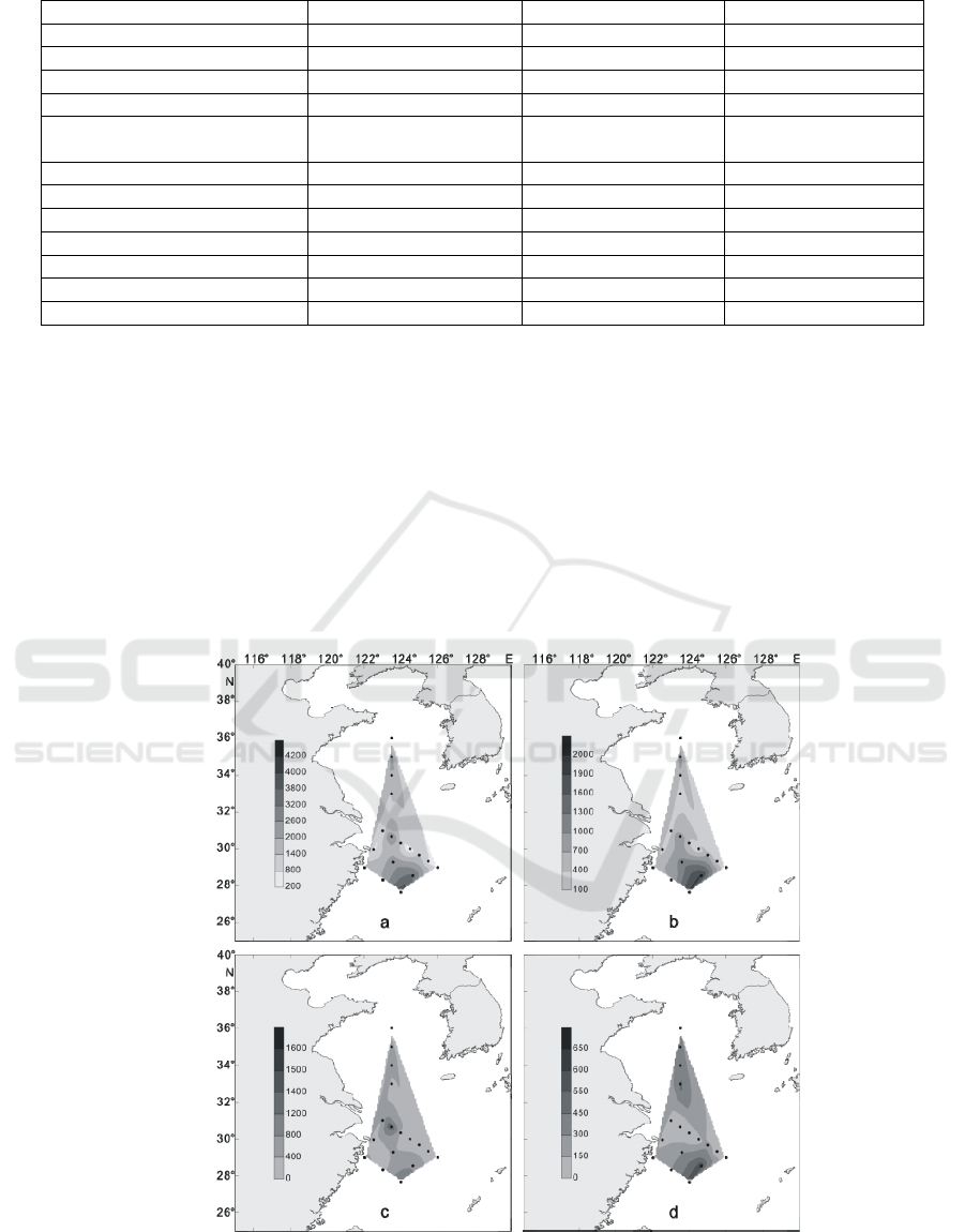
In summer 2016, the cell abundance of LC in the

survey area was between 0.23 ~ 17.62 × 10

cells / L,

with an average of 2.84 × 10

cells / L. Cell

abundance of Emiliania huxleyi was between 0.79 ~

7.4 × 10

cells / L, with an average of 1.04 × 10

cells / L. Cell abundance of Gephyrocapsa oceanica

was between 0.29 ~ 7.6 × 10

cells / L, with an

average of 0.93 × 10

cells / L. Umbellosphaera

tenuis was between 0 ~ 2.22 × 10

cells / L, with an

average of 0.42 × 10

cells / L. (Figure 3)

In summer, the distribution of LC in the study

area is uneven, and a high value suddenly appears at

a certain site in the investigation area. This is due to

the fact that the distribution of LC in summer is not

only affected by light and nutrients, but also

influenced by the interaction of the warm Kuroshio

in the South and the cold water mass of the Yellow

Sea in the north. At the same time, as the largest

diluted water runoff in the coastal areas of China, the

influence of Yangtze River on the distribution of LC

can not be ignored

(Honjo, 1976).



Figure 3: The distribution of living coccolithophores' cell abundance at surface water in summer of 2016 (cells / L, a:

coccolithophores; b: Emiliania huxleyi; c: Gephyrocapsa oceanica; d: Umbellosphaera tenuis)

Community and Distribution of Living Coccolithophores in the Yellow Sea and East China Sea

155



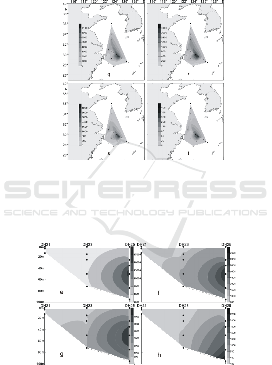
Figure 4: The distribution of living coccolithophores' cell abundance at surface water in winter of 2016 (cells / L, q:

coccolithophores; r: Emiliania huxleyi; s: Gephyrocapsa oceanics; t: Florisphaera profunda)

2.3.3 Vertical Distribution

In summer, LC were mostly located in 35 m, 50 m

and 75 m water layer, the maximum cell abundance

appears in DH25 station of section 1 of 50 m layer

of water, reaching 17.62 × 10

cells / L, and in the

stations of 35 m and 75 m layer, layer respectively

reached 14.83 × 10

cells / L and 12.46 × 10

cells /

L of higher value. Meanwhile, in the section 3 of

PN09 station, there’s a high value of 10.28 × 10

cells / L. (Figures 5-8) Vertical distribution of the

survey area presents a patchy and “bull's eyes”

distribution mode (Zou et al., 2001), a sudden

abundance of high value appears in a water layer in

some stations.



Figure 5: The vertical distribution of living coccolithophores' cell abundance in section 1 in summer of 2016 (cells / L, e:

coccolithophores; f: Emiliania huxleyi; g: Gephyrocapsa oceanica; h: Umbellosphaera tenuis) .

WRE 2021 - The International Conference on Water Resource and Environment

156



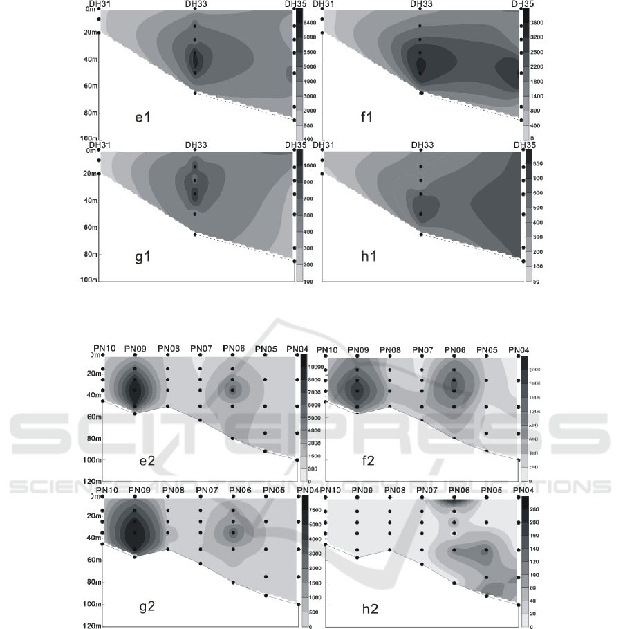
Figure 6: The vertical distribution of living coccolithophores' cell abundance in section 2 in summer of 2016 (cells / L, e1:

coccolithophores; f1: Emiliania huxleyi; g1: Gephyrocapsa oceanica; h1: Umbellosphaera. tenuis).



Figure 7: The vertical distribution of living coccolithophores' cell abundance in section 3 in summer of 2016 (cells / L, e2:

coccolithophores; f2: Emiliania huxleyi; g2: Gephyrocapsa oceanica; h2: Umbellosphaera tenuis).

In the winter of 2016, the LC in the Yellow Sea

and East China Sea were distributed in the 3 water

layers of 25 m, 50 m and 75 m. The maximum

abundance of LC appeared in the 50 m layer of the

PN06 station of section 3, and reached 35.35 × 10

cells / L.At the same time, the 25 m and 75 m layer

of the sation also reached 26.45 × 10

cells / L and

20.67 × 10

cells / L. In addition to the PN06

station, the high values of 8.66 × 10

cells / L and

8.47 × 10

cells / L were achieved at the 55 m layer

of PN09 and the 65 m layer of PN07. Different from

summer, the higher value of the abundance of LC

appeared in the section 4 of the survey area, which

appeared respectively at the 50 m layer of HH13

station and the 35 m layer of the HH14 station, and

the value reached 6.97 × 10

cells / L and 5.56 × 10

cells / L. (Figures 9-12) The vertical distribution of

LC in winter is similar to that in summer, also

showing the characteristics of uneven distribution,

high value abundance will suddenly appear at a

certain water level in some stations.

Community and Distribution of Living Coccolithophores in the Yellow Sea and East China Sea

157



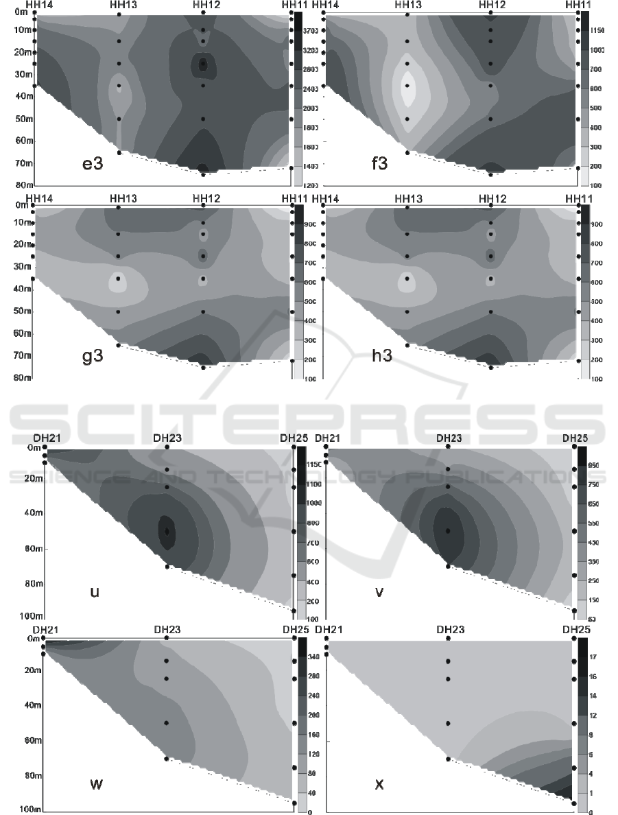
Figure 8: The vertical distribution of living coccolithophores' cell abundance in section 4 in summer of 2016 (cells / L, e3:

coccolithophores; f3: Emiliania huxleyi; g3: Gephyrocapsa oceanica; h3: Umbellosphaera tenuis).



Figure 9: The vertical distribution of living coccolithophores' cell abundance in section 1 in winter of 2016 (cells / L, u:

coccolithophores; v: Emiliania huxleyi; w: Gephyrocapsa oceanica; x: Florisphaera profunda).

WRE 2021 - The International Conference on Water Resource and Environment

158



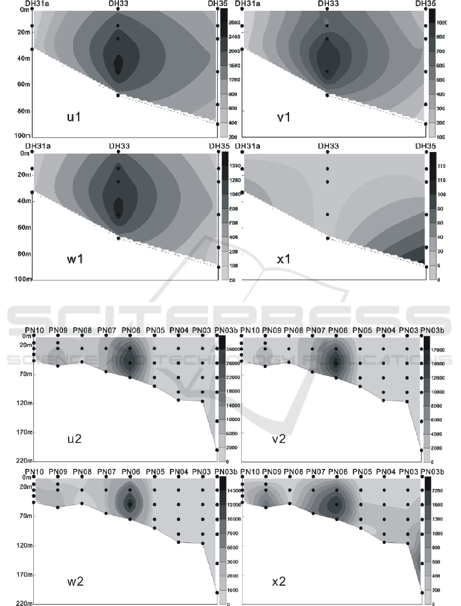
Figure 10: The vertical distribution of living coccolithophores' cell abundance in section 2 in winter of 2016 (cells / L, u1:

coccolithophores; v1: Emiliania huxleyi; w1: Gephyrocapsa oceanica; x1: Florisphaera profunda).



Figure 11: The vertical distribution of living coccolithophores' cell abundance in section 3 in winter of 2016 (cells / L, u2:

coccolithophores; v2: Emiliania huxleyi; w2: Gephyrocapsa oceanica; x2: Florisphaera profunda).

Community and Distribution of Living Coccolithophores in the Yellow Sea and East China Sea

159



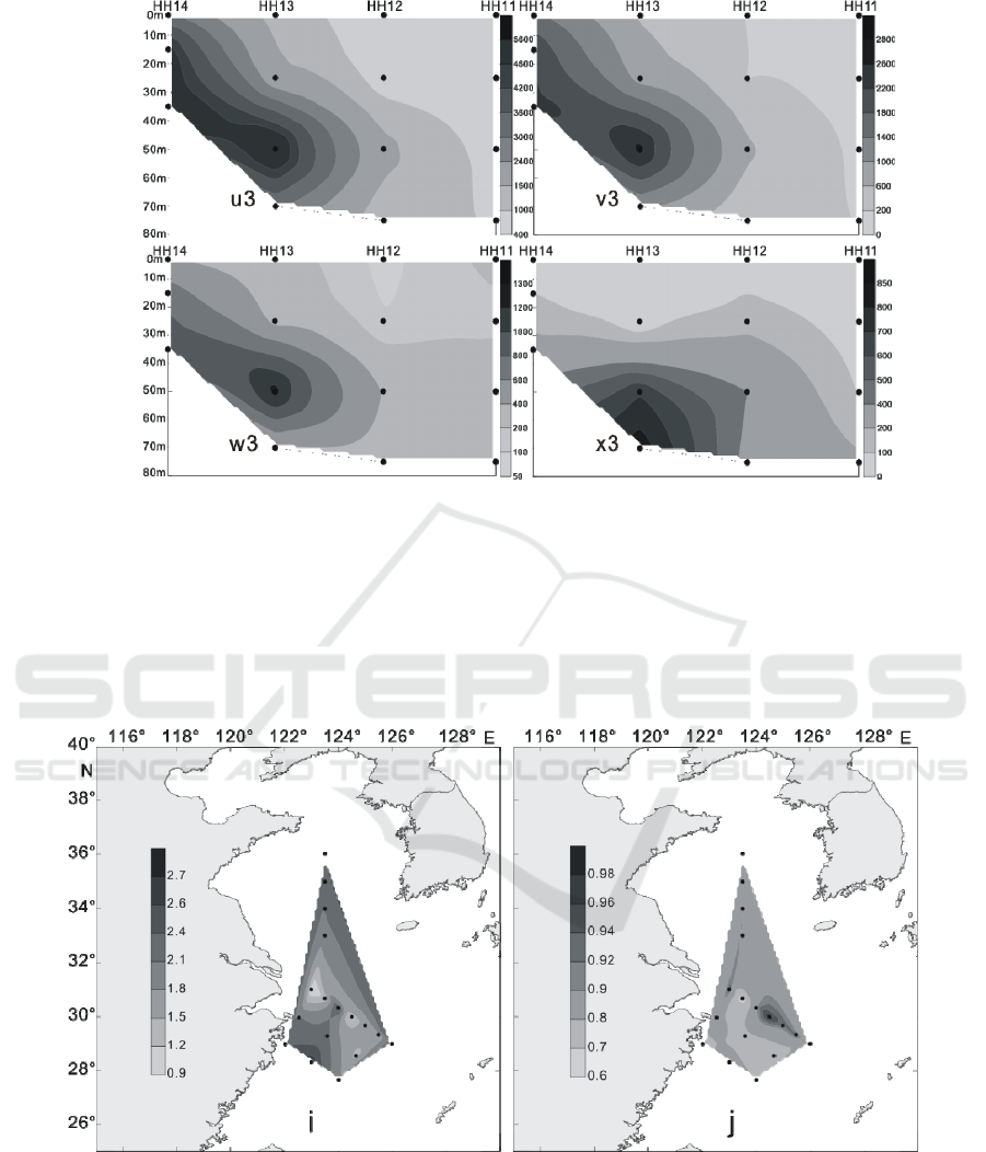
Figure 12: The vertical distribution of living coccolithophores' cell abundance in section 4 in winter of 2016 (cells / L, u3:

coccolithophores; v3: Emiliania huxleyi; w3: Gephyrocapsa oceanica; x3: Florisphaera profunda).

2.3.4 Diversity Index and Evenness

In summer, the community diversity index (Figure

13i) of LC was between 0.72 to 2.35, with an

average of 1.84. The diversity index is higher in the

north and south of the investigation area and the

adjacent sea area, and there is a high value in the

PN08 station in the central area. The evenness index

(Figure 13j) was between 0.49 to 0.99, with an

average of 0.82, which has a higher value in the

central and eastern waters of the study area.



Figure 13: Distribution of Shannon-Wiener diversity index and Pielou evenness index at surface water of survey area in

summer of 2016 (i: Shannon-Wiener diversity index; j: Pielou evenness index).

In the winter of 2016, the species diversity index

(Figure 14y) in the Yellow Sea and East China Sea

was between 1.11~ 2.62, with an average of 1.85.

The highest value of species diversity index appears

in HH12 station and its adjacent waters. The

diversity index of the whole survey area is higher in

the northern, Eastern and southern areas and

adjacent sea areas, and the stations with higher

values are HH12, PN06 and DH35.The distribution

of Pielou evenness index and the distribution of

WRE 2021 - The International Conference on Water Resource and Environment

160

diversity index in the investigation area showed a

more consistent feature, with a value of 0.57~0.95,

with an average value of 0.78 (Figure 14z), which

had a higher value in the middle and adjacent waters

of the investigation area.



Figure 14. Distribution of Shannon–Wiener diversity index and Pielou evenness index at surface water of the survey area in

the winter of 2016(y: Shannon-Wiener diversity index; z: Pielou evenness index).

2.3.5 Distribution of Surface Temperature and

Salinity of the Survey Area

In the summer of 2016, the distribution of surface

temperature and salinity in the Yellow Sea and East

China Sea was shown in figure 15. The surface

temperature of the investigated area is 25.52 ℃ ~

29.99 ℃, with an average value of 28.34 ℃. The

highest value of temperature appeared in the eastern

and southern parts of the investigation area, and the

highest value appeared at DH33 station, with a value

of 29.99 ℃. At the PN10 station closest to the

Yangtze River Estuary, the temperature reaches a

minimum of 25.52 ℃. As can be seen from figure

15o, the trend of surface temperature distribution in

the Yellow Sea and East China Sea area in summer

is from north to south, from nearshore to distant sea,

and the temperature is getting higher and higher.

The salinity of the surface layer in summer survey

area is 22.39~33.69, with an average of 29.96. The

high salinity area appeared in the eastern part of the

survey area, and the highest value appeared at PN04

station, reaching 33.69. At the southern DH35

station, salinity reached a minimum value of 22.39.

As can be seen from figure 15p, the surface salinity

of Yellow Sea and East China Sea in summer is

greatly influenced by the Yangtze River fresh water.

The surface salinity of the near shore is low, and it is

increasing along the direction of fresh water to the

outer sea.

In the winter of 2016, the distribution of surface

temperature and salinity in the Yellow Sea and East

China Sea was shown in figure 16. The surface

temperature of the investigated area is

7.63~22.87 ℃, with an average value of 15.73 ℃.

The highest value of temperature appeared in the

southeastern part of the investigation area, and the

highest value appeared at PN03b station, with a

value of 22.87 ℃. Meanwhile, at the North HH11

station, the temperature reached a minimum of

7.63 ℃. As can be seen from figure 16E, the surface

temperature distribution trend in winter is similar to

that in summer, which is from north to south, from

near shore to far sea, and the temperature is getting

higher and higher.

The salinity of the surface layer in winter survey

area is 27.06~34.58, with an average of 33.24. The

high salinity area appeared in the eastern part of the

survey area, and the highest value appeared at PN03

station, reaching 34.58. At the DH21 station near the

Gulf of Hangzhou, salinity reached a minimum

value of 27.06. As can be seen from figure 16F, the

surface salinity in winter is still influenced by inland

runoff, and the surface salinity is low in the near

shore, increasing along the direction of fresh water

to the outer sea.

Community and Distribution of Living Coccolithophores in the Yellow Sea and East China Sea

161



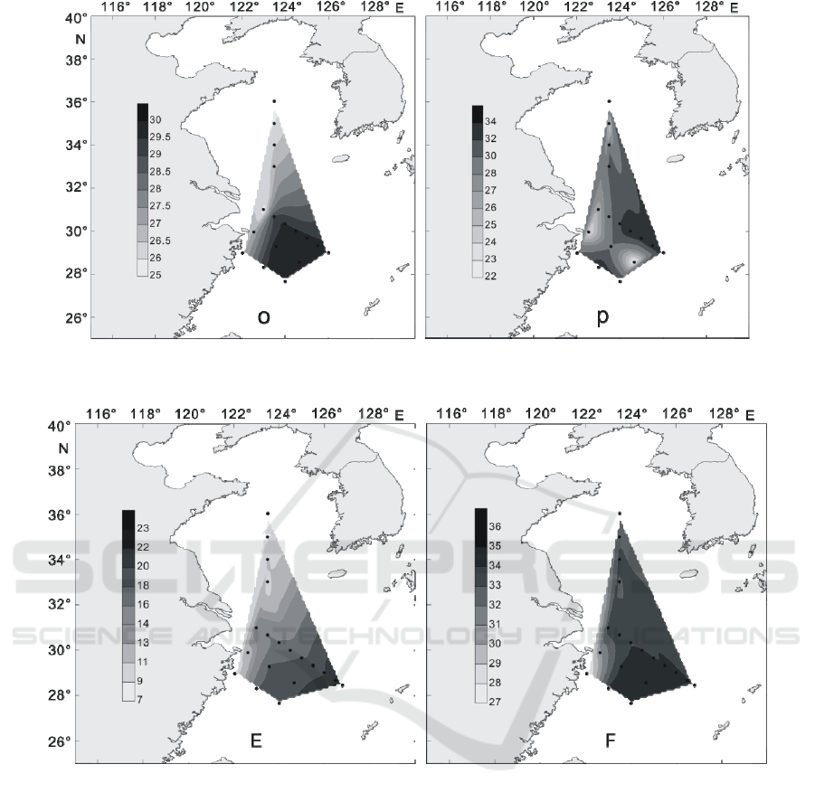
Figure 15. The distribution of temperature and salinity in surface layer of the survey area in summer of 2016 (o: the

distribution of temperature in surface layer (℃); p: the distribution of salinity in surface layer)

Figure 16: The distribution of temperature and salinity in surface layer of the survey area in winter of 2016 (E: the

distribution of temperature in surface layer (℃); F: the distribution of salinity in surface layer).

3 SUMMARY

This paper mainly studied the community and

distribution of LC in the summer of 2016 (July 20th

to September 1st) and winter (December 23rd to

February 5th) of the Yellow Sea and East China Sea

in China.

21 kinds of living coccolithophores were found in

the survey area in summer, most of them are

heterococcolithophores, only a few of

holococcolithophores. The dominant species were

Emiliania huxleyi, Gephyrocapsa oceanica,

Umbellosphaera tenuis, Florisphaera profunda,

Helicopontosphaera carteri and Umbilicosphaera

sibogae. The cell abundance of LC in the survey

area was between 0.23 ~ 17.62 × 10

cells / L, with

an average of 2.84 × 10

cells / L.The high value

areas of these dominant species usually appear in the

southern part of the investigation area and the

surrounding waters. This is due to the fact that the

distribution of LC is not only affected by light and

nutrients, but also influenced by the interaction of

the warm Kuroshio in the South and the cold water

mass of the Yellow Sea in the north

(Yang & We i,

2003). At the same time, the influence of the

Yangtze River is very significant.

WRE 2021 - The International Conference on Water Resource and Environment

162

20 kinds of living coccolithophores were found in

the survey area in winter, and Most of them are

heterococcolithophores. The dominant species were

E. huxleyi, G. oceanica, F. profunda, U. tenuis, S.

pulchra and U. sibogae. The cell abundance of LC

was between 0.12 ~ 35.35 × 10

cells / L, with an

average of 3.84 × 10

cells / L. Compared with

summer, the abundance of LC increased greatly in

winter, but the species of the dominant species

changed little. The high value area of the abundance

of LC appeared in the middle and eastern waters,

and its abundance coverage is much wider than that

in summer.

The reasons for the difference between summer

and winter were mainly due to the effect of strong

monsoon in the sea area in winter, and the effect of

upwelling in the shelf of Yellow Sea and East China

Sea was remarkable. The upwelling transported

nutrients from bottom of the sea water to the upper

water body in a certain area

(Yu et al., 2006)., and

the warm Kuroshio water also changed the living

environment of LC to a great extent. Together, they

give the necessary nutrients and environment for the

growth of the algae, resulting in higher cell

abundance.

ACKNOWLEDGMENTS

We are grateful to the research vessel Xiang Yang

Hong 01, for providing the seawater samples. The

research was funded by National Key R&D Program

of China (2016YFC1401906).

REFERENCES

Billard, C., & Inouye, I. (2004). What is new in

coccolithophore biology? In: Coccolithophore: from

molecular processes to global impact. Thierstein H R,

Young J R, eds. Berlin: Springer-Verlag Berlin, 35-37.

Bollmann, J., Cortés, M. Y., & Haidar, A. T. (2002).

Techniques for quantitative analyses of calcareous

marine phytoplankton. Marine Micropaleontology, 44,

163-185.

Heimdal, B. R. (1993). Modern coccolithophorid. In:

Tomas C R, eds. Identifying Marine Phytoplankton.

United Kingdom: Academic Press, 147-247.

Honjo, S. (1976). Coccoliths production, transportation,

sedimentation. Marine Micropaleontology, 1, 65-79.

Jordan, R. W. & Kleijne, A. (1994). A classification

system for coccolithophores. In: Winter A, Siesser W

G, eds. Coccolithophores. United Kingdom:

Cambridge University Press, 83-105.

Sun, J. (2007). Organic carbon pump and carbonate

counter pump of living coccolithophorid. Advances in

earth science, 22(12), 1231-1239.

Winter, A., & Siesser, G. (1994). Atlas of

coccolithophores. In: Winter A and Siesser W G, eds

Coccolithophores. Cambridge: Cambridge University

Press, 107-159.

Yang, T. N., & Wei, K. Y. (2003). How many coccoliths

are there in a coccosphere of the extant

coccolithophorids? A compilation. Journal of

Nannoplankton Research, 25, 7-15.

Yu, F., Zhang, Z., Diao, X. Y., Guo, J. X., & Tang, Y. X.

(2006). Analysis of evolution of the Huanghai Sea

Cold Water Mass and its relationship with adjacent

water. Acta Oceanologica Sinica, 28(5), 26-34.

Zou, E. M., Guo, B. H., Tang, Y. X., Li, Z. X., & Li, X. Z.

(2001). A number of hydrological characteristics and

circulation analysis in Southern Yellow Sea and

Northern East China Sea in summer. Oceanologia et

Limnologia Sinica, 32(3), 340-348.

Community and Distribution of Living Coccolithophores in the Yellow Sea and East China Sea

163