An Evaluation of Post-Processed Monthly Precipitation Forecasts

from Different Models in Guangdong, China

Shuai Xie

1,2,3

, Tao Zhou

1,2,3

, Xiaoqi Zhang

1,2,3

, Yongqiang Wang

1,2,3,*

and Hang Lin

1,2,3

Water Resources Department, Changjiang River Scientific Research Institute, Wuhan 430010, China

Hubei Key Laboratory of Water Resources and Eco-Environmental Sciences, Wuhan 430010, China

Research Center on the Yangtze River Economic Belt Protection and Development Strategy, Wuhan 430010, China

Keywords: Monthly precipitation forecasts, Post-processing, Bayesian joint probability, Bayesian model averaging

Abstract: Monthly precipitation forecasts are important in water resources management. In this study, the monthly

precipitation forecasts of the future 1-6 months generated by five different national weather services are

corrected by Bayesian Joint Probability (BJP) method and merged by Bayesian Model Averaging (BMA)

method. The predictive performance of corrected and merged forecasts is evaluated and compared with the

climatology forecasts in 26 meteorological stations in Guangdong, China. The results demonstrate that the

BJP-corrected forecasts are more reliable and narrower than the climatology forecasts and The BMA

method can further improve the forecasting reliability and accuracy in the BJP-BMA framework. The

forecasting skill of the BJP-BMA framework varies significantly with different forecast lead time (FLT).

When FLT is 1 month, the raw forecasts are informative, and the BJP-BMA framework can generate

significantly better forecasts than the climatology forecasts with respect to the forecasting accuracy,

reliability and sharpness. When FLT is greater than 1, the information contained in raw forecasts are

limited, but the BJP-BMA can still generate narrower and more reliable forecasts. In summary, the proposed

BJP-BMA framework can extract useful information in the raw forecasts and generate more practical

monthly precipitation forecasts.

1 INTRODUCTION

Monthly precipitation forecasts are of great

importance in hydrological forecasts, water

resources management and decision making in many

climate-sensitive sectors (Li et al., 2021; Wang et al.,

2019a). Many studies demonstrate that the climate

change has resulted in the increasing frequency of

extreme rainfall and extreme drought, which further

enhances the demands for reliable and high-

resolution monthly precipitation forecasts (Kao and

Ganguly, 2011; O’Gorman, 2015; Schepen et al.,

2018).

The methods used to generate monthly

precipitation forecasts can be broadly divided into

two groups: 1) data-driven models and 2) general

circulation models (GCMs) (Li et al., 2021). The

data-driven models are often proposed to model the

relationship between climate factors and monthly

precipitations (Li et al., 2021; Peng et al., 2014).

However, the forecasts obtained from data-driven

models are often deterministic, which are inadequate

in comparison with the ensemble forecasts (Duan et

al., 2019; Li et al., 2019). In comparison with data-

driven models, GCMs, which produce monthly

outlooks of atmospheric and oceanic conditions and

fluxes, are proposed by many national weather

services (NWSs) (Johnson et al., 2019; Molteni et

al., 2011; Saha et al., 2014; Zhao et al., 2017). For

example, the European Centre for Medium-Range

Weather Forecasts (ECMWF) operated its System 4

in 2011 and has operated the newest Seasonal

Forecast System 5 (SEAS5) since 2017 (Wang et al.,

2019a). Though the GCMs can produce ensemble

forecasts, they have their own deficiencies, which

make them unsuitable for practical application. For

example, the forecasts generated by GCMs are

usually biased and not always “skillful” (Zhao et al.,

2017). Therefore, many post-processing methods

are applied and obtained good performance (Wang

et al., 2019a; Wang et al., 2019b; Zhao et al., 2017).

Many NWSs have operated their seasonal

forecast systems and the post-processed forecasts are

skillful and useful (Bennett et al., 2016; Crochemore

Xie, S., Zhou, T., Zhang, X., Wang, Y. and Lin, H.

An Evaluation of Post-processed Monthly Precipitation Forecasts from Different Models in Guangdong, China.

In Proceedings of the 7th International Conference on Water Resource and Environment (WRE 2021), pages 76-87

ISBN: 978-989-758-560-9; ISSN: 1755-1315

et al., 2016). Current post-processing methods are

always used to process forecasts generated from one

NWS, but different NWSs may offer different

forecasting information (Mohanty et al., 2021; Zhou

et al., 2020). Therefore, how to combine the

strengths of individual models still needs to be

investigated in order to achieve better forecasting

performance. In this study, a post-processing

framework, which can combine the forecasts from

different NWSs, is proposed to correct and merge

forecasts of different NWSs. The framework is

applied and evaluated in terms of its predictive

performance in Guangdong, China.

2 STUDY AREA AND DATA

2.1 Study Area and Observed Data

In order to evaluate and compare the predictive

performance of post-processed monthly precipitation

forecasts from different models (i.e. different

NWSs), the forecasting precipitation products during

future 1-6 months are post-processed and evaluated

over 26 meteorological stations in Guangdong,

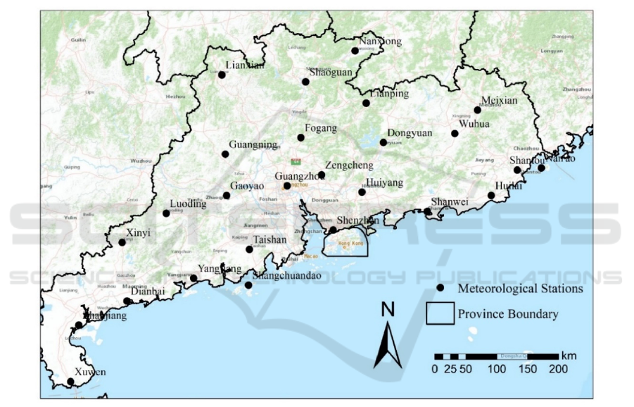
China. The 26 meteorological stations are shown in

Figure 1. The locations and names of the stations are

shown in Table 1.

Figure 1: Study area and meteorological stations.

An Evaluation of Post-processed Monthly Precipitation Forecasts from Different Models in Guangdong, China

Table 1: The locations and names of meteorological stations.

Station

Abbreviated

name

Longitude Latitude Station

Abbreviated

name

Longitude Latitude

Xuwen XW 110.18 20.33 Zengcheng ZC 113.83 23.33

Zhanjiang ZJ 110.3 21.15 Fogang FG 113.53 23.87

Dianbai DB 111 21.5 Shaoguan SG 113.6 24.68

Xinyi XY 110.93 22.35 Nanxiong NX 114.32 25.13

Yangjiang YJ 111.97 21.83 Lianping LP 114.48 24.37

Luoding LD 111.57 22.77 Dongyuan DY 114.73 23.8

Shangchuandao SCD 112.77 21.73 Huiyang HY 114.42 23.08

Taishan TS 112.78 22.25 Shanwei SW 115.37 22.8

Gaoyao GY 112.45 23.03 Wuhua WH 115.77 23.93

Guangning GN 112.43 23.63 Meixian MX 116.1 24.27

Lianxian LX 112.38 24.78 Huilai HL 116.3 23.03

Guangzhou GZ 113.33 23.17 Shantou ST 116.68 23.4

Shenzhen SZ 114 22.53 Nan'ao NA 117.03 23.43

The observed daily precipitation of the 26

meteorological stations are obtained online

(http://data.sheshiyuanyi.com/WeatherData/) and

processed to monthly data. The data are all available

from 1984 to 2019 and the data from 1993 to 2016

are used in this study in order to consist with the

forecasts data.

2.2 Monthly Precipitation Forecasts

In seasonal forecast systems, the models are

initialized with the initial conditions of the earth

system. However, due to the imperfect knowledge of

the initial conditions, many approximations are

made and result in uncertainties, which are

dependent on the choice of model. Therefore,

different models may have different predictive skills.

In order to combine outputs from several models, the

Copernicus Climate Change Service (C3S) provides

a multi-system seasonal forecast service, where data

are obtained from several state-of-the-art seasonal

prediction systems developed, implemented and

operated at forecast centers in several countries. The

centers include ECMWF, The UK Met Office

(UKMO) and Météo-France (MF), Deutscher

Wetterdienst (DWD), Centro Euro-Mediterraneo sui

Cambiamenti Climatici (CMCC) and so on. In these

studies, the forecasting precipitations for the future

1-6 months from 1993 to 2016, which are generated

by ECMWF, UKMO, MF, DWD and CMCC, are

used. The data can be obtained on

https://cds.climate.copernicus.eu/cdsapp#!/dataset/se

asonal-monthly-single-levels?tab=form.

3 METHODOLOGY

3.1 Modelling Framework

Based on the observed data and the monthly

precipitation forecasts, the post-processing and

merging methods are applied in the way shown in

Figure 2. Firstly, due to the forecasts are gridded

data, the forecasts over 26 specific stations are

computed by a two-dimensional interpolation

method. Moreover, due to the post-processing

method will generate ensemble forecasts, the means

of the original forecasts are used in the post-

processing process. Then, the Bayesian Joint

Probability (BJP) method is used to correct the

original forecasts based on the observations and

generate corrected ensemble forecasts. Finally, the

corrected forecasts are merged by the Bayesian

Model Averaging (BMA) method. In order to assess

the impact of the BJP and BMA methods, the

climatology forecasts, which are randomly sampled

from the observations month by month, are

employed as reference forecasts. It should be noted

that the models operated by five NWSs are denoted

by CMCC, DWD, MD, UKMO and ECMWF

models in Figure 2 and following contents.

WRE 2021 - The International Conference on Water Resource and Environment

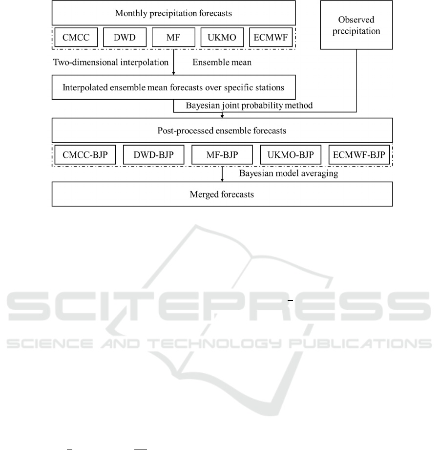
Figure 2: Modelling framework.

3.2 Bayesian Joint Probability

Many studies have demonstrated that the post-

processing can improve the reliability and accuracy

of precipitation forecasts (Bennett et al., 2016;

Crochemore et al., 2016; Wang et al., 2019a).

Among the post-processing methods, the BJP

method has been widely used because it can not only

correct the bias but also ensure the corrected

forecasts are not worse than the climatology

forecasts (Robertson and Wang, 2012; Schepen and

Wang, 2014; Wang, 2008; Wang et al., 2009; Zhao

et al., 2016). In this study, the BJP is also employed.

Before the BJP, the data need to be transformed

into normalized data and the log-sinh transformation

is implemented (Wang et al., 2019b). The log-sinh

transformation can be expressed as in Equation (1).

𝑧̂





𝜆

log



sinh



ℇ

𝜆𝑧



𝑐



(1)

where 𝑧



and 𝑧̂



are original and transformed data

respectively, ℇ and 𝜆 are transformation parameters,

𝑐 is a scaling factor used to make the scaled 𝑧



/𝑐 has

a similar range in different applications. After the

transformation, the data should follow a normal

distribution and the maximum likelihood method

can be applied to optimize the parameters given a

dataset (Wang et al., 2019b). After the parameters

optimization, the data can be transformed by

Equation (1) and back-transformed by the following

Equation (2):

𝑧





𝑐

𝜆

arcsinh



exp



𝜆𝑧̂





ℇ

(2)

Denoting the original forecasting precipitation as

𝑦



, the corresponding observation as 𝑦



, the BJP is

used to obtain the corrected 𝑦





based on the prior

and posterior information included in the original

forecasts and observations. Through the data

transformation, 𝑦



and 𝑦



are transformed to

normalized 𝑧



and 𝑧



. Assuming 𝑧



and 𝑧



are

normally-distributed and the 𝒛



𝑧



𝑧





is drawn

from a bivariate normal distribution as in Equation

(3).

𝒛

𝑧



𝑧



~𝑁𝝁,𝚺 (3)

where 𝝁 is the mean values of two transformed

variables and 𝚺 is a covariance matrix.

Given a transformed dataset 𝑫𝒛



𝑡



,𝑡

1,2,…𝑛, where n is the number of samples, the

posterior of the model parameters can be written as

the following Equation (4) according to Bayes’

theorem.

𝑝



𝝁,𝚺

𝑫



∝𝑝



𝝁,𝚺



𝑝



𝑫

𝝁,𝚺



𝑝



𝝁,𝚺



𝑝𝒛𝑡|𝝁,𝚺







(4)

An Evaluation of Post-processed Monthly Precipitation Forecasts from Different Models in Guangdong, China

where 𝑝



𝝁,𝚺



is the prior and 𝑝



𝑫

𝝁,𝚺



is the

likelihood. Due to the posterior in equation (4) is not

a standard distribution and does not allow analytical

integration, the technique of Markov Chain Monte

Carlo sampling is used to draw parameter values. In

this study, the Gibbs MCMC sampling is used to

draw 1000 sets of parameter values (Wang et al.,

2019a).

Given a transformed forecasting value 𝑧



𝑡

∗

 at a

specific time 𝑡

∗

, a corrected forecasting value 𝑧





𝑡

∗



is obtained by sampling from 𝑝



𝑧





𝑡

∗

|

𝑧





𝑡

∗



,𝝁,𝚺



Then, the sampled value are back-transformed to

original value by Equation (2). For each set of

parameters, one value is sampled and therefore there

are 1000 values in the ensemble forecasts generated

from BJP.

3.3 Bayesian Model Averaging

The BMA, which gives greater weights to better

models based on their probabilistic forecasting

performance, is a method used for merging forecasts

from multiple models. The detailed procedure of

BMA can be found in previous studies (Bennett et

al., 2016; Schepen et al., 2016; Wang et al., 2012).

The probabilistic forecasting performance is

evaluated by the predictive density at the observed

value.

Given a group of models 𝑀



(𝑘1,2,…,𝐾), the

predictive density after BMA is a weighted average

of predictive densities of K models as in Equation

(5).

𝑓





𝑌





𝑤



𝑓

𝑌



|𝑀









(5)

where 𝑤



is the weight of kth model, 𝑌



is the

observed value at ith sample point, and 𝑓𝑌



|𝑀



 is

the predictive density of model 𝑀



The weights in BMA can be optimized by the

maximum a posterior method (Bennett et al., 2016;

Wang et al., 2012). Denoting the weights as 𝒘



𝑤



,𝑤



,…,𝑤







, the posterior is as follows in

Equation (6).

𝑝



𝒘

𝒀,𝑴



∝𝑝



𝒘



∗𝑝𝒀|𝒘,𝑴

(6)

where 𝑝



𝒘



is the prior, 𝑝𝒀|𝒘,𝑴 is the likelihood,

𝒀 is the observation vector and 𝑴 is the set of all

models. The symmetric Dirichlet distribution prior is

employed and the likelihood can be calculated by

the following Equation (7).

𝑝



𝒀

𝒘,𝑴





𝑓





𝑌











𝑤



𝑓

𝑌



|𝑀

















(7)

where n is the number of sample points. Based on

the prior and likelihood, the posterior in Equation (6)

can be calculated. Then the weights can be

optimized by an iterative expectation-maximization

algorithm. Noted that the sum of the weights is 1,

the merged forecasts can be obtained by sampling

from the ensemble forecasts from different models

by their weights.

3.4 Evaluation Criteria

In this study, a leave-one-month-out cross-validation

procedure is used to generate corrected results by

BJP and merged results by BMA. The forecast

performance of the corrected and merged results are

evaluated in different aspects in this

study(Crochemore et al., 2016; Wang et al., 2019a):

1) the continuous ranked probability score (CRPS),

which reflect the overall accuracy of the ensemble

forecasts(Gneiting et al., 2005; Renard et al., 2010);

2) the score based on the probability integral

transform (PIT) diagram (PITS), which reflect the

reliability and is obtained by calculating the area

between the PIT diagram and the 1:1 diagonal

(Jordan et al., 2017); and 3) the score calculated by

averaging the 90% interquantile range (i.e. the

difference between the 95

and 5

percentiles)

(IQRS), which reflect the sharpness (Crochemore et

al., 2016). The detailed calculating procedure can be

found in corresponding studies and not listed here.

Forecast skill of the corrected and merged

forecasts is assessed by comparing the forecast

performance of a given system with the performance

of a reference forecast. The skill score is calculated

by the following Equation (8).

𝑆𝑘𝑖𝑙𝑙1 

𝑆𝑐𝑜𝑟𝑒



𝑆𝑐𝑜𝑟𝑒



  100%

(8)

where 𝑆𝑐𝑜𝑟𝑒



is the CRPS, PITS or IQRS of the

given system (i.e. BJP or BMA) and 𝑆𝑐𝑜𝑟𝑒



is the

score of the reference forecasts. The forecast skill

corresponding to CRPS, PITS and IQRS are noted

CRPSS, PITSS, IQRSS.

WRE 2021 - The International Conference on Water Resource and Environment

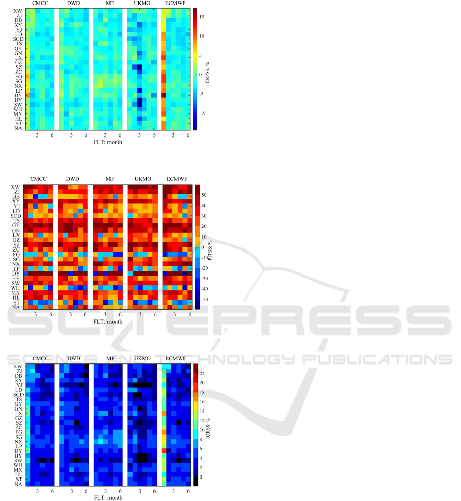
Figure 3: CRPSS of the BJP corrected ensemble forecasts.

Figure 4: PITSS of the BJP corrected ensemble forecasts.

Figure 5: IQRSS of the BJP corrected ensemble forecasts.

4 RESULTS AND DISCUSSION

4.1 Forecast Performance of the

Corrected Ensemble Forecasts by

BJP

As introduced above, the BJP method is used to post-

process the raw forecasts. In order to evaluate the

forecast performance of the BJP corrected ensemble

forecasts, the skill scores (CRPSS, PITSS, IQRSS)

are calculated with the climatology forecasts as

reference forecasts. The CRPSS, PITSS, and IQRSS

results are shown in Figure 3, Figure 4 and Figure 5

respectively. In addition, the statistics of these three

scores over 26 stations are shown in Table 2.

It can be seen from Figures 3-5 and Table 2 that

the corrected forecasts generated by BJP can

outperform the climatology forecasts in most cases

and the improvement is especially significant when

FLT is 1 month. The mean values of PITSS and

IQRSS are greater than 0 for all models and all FLTs,

which means the corrected forecasts are more

reliable and narrower. However, the mean values of

CRPSS are less than 0 for corrected forecasts based

on MF and UKMO models with all FLTs and for

those based on CMCC, DWD and ECMWF models

with FLT greater than 1, which means the BJP-

corrected forecasts are less accurate. Figure 4

displays the PITSS in different forecasting cases. It

is obvious that in most cases the PITSS is greater

than 0, which means the corrected forecasts are more

reliable than the climatology forecasts. However, in

some stations (FG, WH, ST), the forecasting

reliability decreases. Figure 5 shows that the IQRSS

is greater than 0 in most cases, which means that the

information included in the raw forecasts can narrow

the forecasting width, which makes the forecasts

more practical. In terms of the comparison of

different models, it is also obvious that the ECMWF

model has an overall better performance with respect

to the CRPSS and IQRSS. When FLT is 1 month,

the mean CRPSS and IQRSS are 8.10% and 12.73%

for ECMWF-based corrected forecasts, which

outperforms those based on other models.

In summary, the BJP corrected ensemble

forecasts are more reliable and practical than the

climatology forecasts. With respect to the

forecasting accuracy, the CMCC, ECMWF-based

corrected forecasts are more accurate when FLT is 1

month. In terms of the comparison of different

models, the ECMWF models are more skillful than

the other models when FLT is 1 month. In terms of

the FLT, it can be found that the improvement of

forecasting performance is more significant when

FLT is 1 month.

An Evaluation of Post-processed Monthly Precipitation Forecasts from Different Models in Guangdong, China

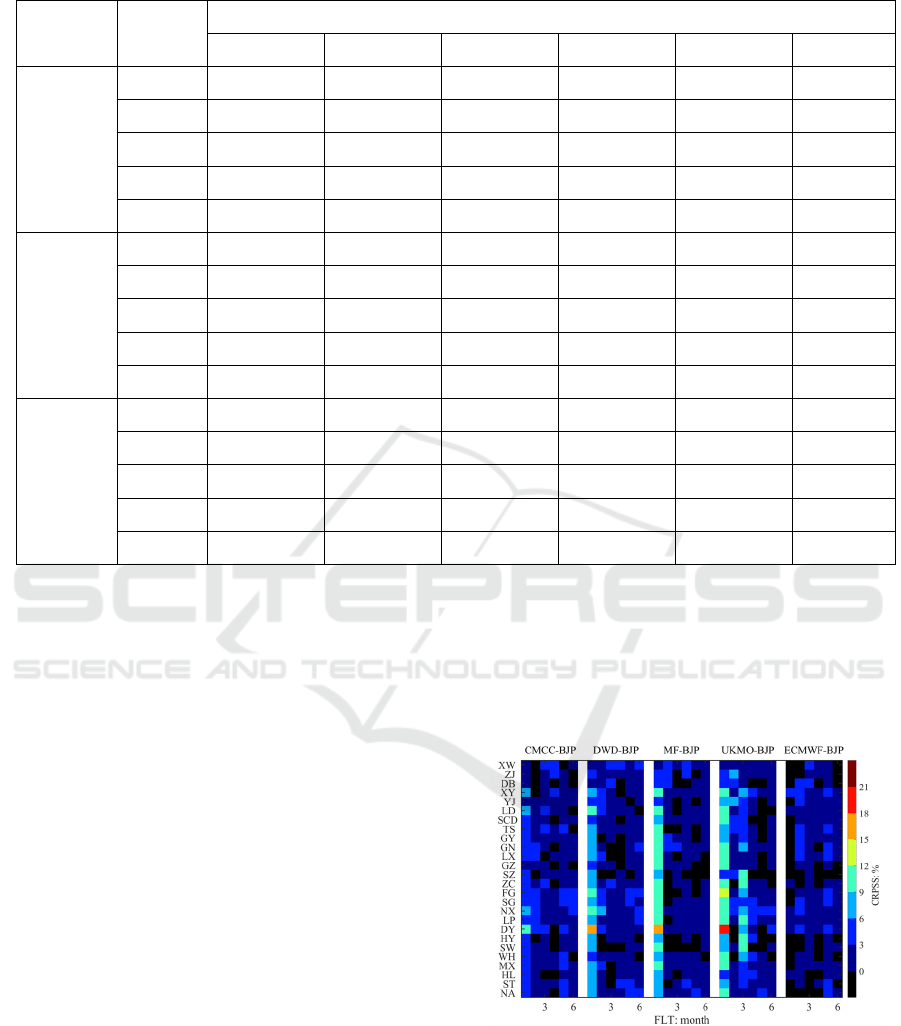
Table 2: Mean values and standard deviations of CRPSS, PITSS and IQRSS after BJP over all stations.

Scores NWS

FLT: months

1 2345 6

CRPSS: %

CMCC 3.09±2.16 -2.43±2.05 -2.40±0.98 -1.90±1.22 -3.14±1.09 -2.92±0.94

DWD 0.22±1.29 -2.72±1.33 -1.51±1.69 -2.29±1.20 -2.53±0.99 -2.94±0.87

MF -1.24±1.49 -1.68±1.86 -0.90±1.43 -2.93±1.20 -1.00±1.42 -2.52±1.39

UKMO -1.76±1.47 -2.72±2.37 -6.17±3.87 -2.87±1.30 -1.39±1.04 -2.73±1.31

ECMWF 8.10±2.95 -2.45±1.84 -1.80±1.27 -1.82±1.39 -3.07±1.00 -1.94±1.26

PITSS: %

CMCC 33.2±22.1 16.9±36.5 16.8±27.8 18.4±27.1 15.6±30.2 17.7±29.1

DWD 26.6±26.6 20.0±26.8 24.3±20.1 14.8±31.9 10.8±32.2 24.4±24.6

MF 32.6±20.4 20.3±25.2 18.2±24.5 14.9±33.5 12.0±35.5 11.3±29.1

UKMO 33.0±17.6 18.7±26.2 16.8±29.3 18.8±28.9 20.7±25.5 22.7±24.2

ECMWF 25.3±29.8 27.7±26.9 18.0±29.6 14.3±36.0 8.7±42.8 25.4±26.8

IQRSS: %

CMCC 8.30±1.65 4.08±1.66 3.81±0.97 2.67±1.38 2.63±1.20 2.90±1.28

DWD 5.17±1.12 3.79±1.33 3.61±1.47 2.84±1.52 2.87±1.50 2.59±1.51

MF 4.33±1.31 3.95±1.52 4.41±1.38 2.60±1.37 3.84±1.83 3.38±1.90

UKMO 3.83±1.47 3.59±2.39 1.24±2.01 1.67±1.32 2.99±1.62 2.73±1.55

ECMWF 12.73±2.55 3.43±1.68 3.90±1.25 2.97±1.63 2.93±1.38 3.42±1.05

4.2 The Impact of the BMA Method

The BMA method is used to merge the corrected

forecasts generated by CMCC-BJP, DWD-BJP, MF-

BJP, UKMO-BJP and ECMWF-BJP models, each of

which means the combination of a NWS model and

the BJP method. In order to evaluate the impact of

the BMA method, the merged forecasts of the BJP-

BMA framework are compared with the BJP

corrected forecasts. The CRPSS, PITSS, and IQRSS

results are shown in Figure 6, Figure 7 and Figure 8

respectively. The statistics of these three scores over

26 stations are shown in Table 3.

It can be seen from Figures 6-8 and Table 3 that

the BJP-BMA framework outperforms a single

model in most cases. It is clear that the CRPSS is

greater than 0 is most cases (Figure 6), which means

the BMA can improve the forecasting accuracy.

However, the mean CRPSSs are near 0 (Table 3),

which means the improvement is not significant.

The BMA has different impact for different FLTs.

When FLT is 1 month, the BJP-BMA framework

has better performance than the CMCC-BJP, DWD-

BJP, MF-BJP and UKMO-BJP models but worse

than the ECMWF-BJP. When FLT is greater than 1,

the BJP-BMA has better performance than all five

BJP-based models. In terms of the predictive

sharpness, the merged forecasts are narrower than

the corrected forecasts of four model (CMCC-BJP,

DWD-BJP, MF-BJP, UKMO-BJP), which can be

seen in Figure 8. In addition, the merged forecasts

are more reliable than the corrected forecasts in most

cases (Figure 7).

Figure 6: CRPSS of the BMA merged forecasts based on

the corrected forecasts.

WRE 2021 - The International Conference on Water Resource and Environment

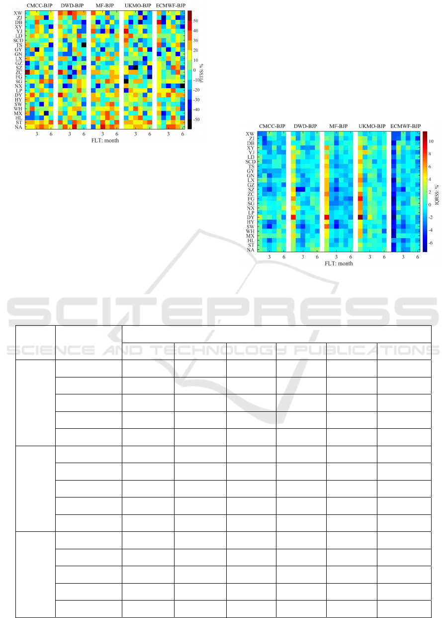
Figure 7: PITSS of the BMA merged forecasts based on

the corrected forecasts.

Due to the different performance of five BJP-

based models with different FLTs, the impact of

BMA varies significantly for different FLTs. When

FLT is 1 month, the BMA can improve the

forecasting accuracy and narrow the forecast width

of four models (i.e. CMCC-BJP, DWD-BJP, MF-

BJP and UKMO-BJP models) but has opposite

impact when compared with the ECMWF-BJP

model. This is because the ECMWF-BJP model has

significantly better performance than the other four

models (Table 2) and and the other four models

cannot offer more information to the merged

forecasts. When FLT is greater than 1 month, due to

the five models have similar performance in terms of

the accuracy and sharpness, the BMA widen the

forecasts and improve the forecasting accuracy. But

the mean values of CRPSS and IQRSS are near 0,

which means the change is not significant. With

respect to the reliability, the BMA can significantly

improve the forecasting reliability in most cases.

Figure 8: IQRSS of the BMA merged forecasts based on

the corrected forecasts.

Table 3: Mean values and standard deviations of CRPSS, PITSS and IQRSS after BMA over all stations.

Scores Base model

FLT: months

1 2 3 4 5 6

CRPSS:

CMCC-BJP 4.49±1.99 1.80±2.07 1.88±1.46 0.55±1.46 2.40±1.48 1.46±1.79

DWD-BJP 7.24±2.73 2.10±1.88 1.01±1.52 0.94±1.27 1.81±1.36 1.49±1.37

MF-BJP 8.65±3.01 1.09±1.73 0.42±1.49 1.55±1.34 0.33±1.07 1.09±0.99

UKMO-BJP 9.02±3.30 2.08±2.06 5.27±3.27 1.49±1.48 0.71±1.41 1.29±1.35

ECMWF-BJP -0.74±1.74 1.83±2.05 1.31±1.28 0.48±1.21 2.33±1.41 0.52±1.38

PITSS:

CMCC-BJP 4.3±17.7 3.6±19.7 3.8±18.3 6.7±17.7 1.9±18.0 0.1±19.6

DWD-BJP 13.2±15.9 2.6±17.5 -4.5±20.3 9.3±19.5 7.3±16.4 -7.3±19.3

MF-BJP 6.4±18.4 2.5±17.2 2.7±17.3 9.6±17.9 5.2±17.5 8.5±15.6

UKMO-BJP 5.4±24.5 4.3±17.1 3.3±20.2 6.1±18.8 -3.3±18.3 -5.2±18.8

ECMWF-BJP 13.4±16.1 -8.2±15.2 2.3±17.4 10.0±14.6 6.7±18.9 -9.4±18.7

IQRSS:

CMCC-BJP 0.13±1.50 -1.05±1.70 -1.62±1.64 -0.78±1.01 -0.06±1.31 -0.50±1.37

DWD-BJP 3.43±1.92 -0.75±1.85 -1.42±1.70 -0.96±0.82 -0.31±1.03 -0.18±1.18

MF-BJP 4.27±2.05 -0.91±1.18 -2.26±1.29 -0.70±1.03 -1.33±0.74 -1.00±1.03

UKMO-BJP 4.75±2.38 -0.55±1.65 1.01±1.25 0.24±0.93 -0.44±0.84 -0.32±1.14

ECMWF-BJP -4.96±1.37 -0.37±1.67 -1.72±1.40 -1.10±0.98 -0.36±0.82 -1.03±1.34

An Evaluation of Post-processed Monthly Precipitation Forecasts from Different Models in Guangdong, China

Figure 9: CRPS, PITS and IQRS of the merged forecasts.

4.3 The Forecasting Skill of the

Merged Forecasts

After the BJP and BMA, the forecasting

performance of the merged forecasts is evaluated

and shown in Figure 9. It is obvious that the CRPS

and IQRS varies significantly over different stations.

This is because the CRPS and IQRS are related with

the range of observations and the precipitations over

different stations are significantly different. In terms

of the reliability, the PITS are all below 0.022,

which means the forecasts are very reliable.

The merged forecasts are also compared with the

climatology forecasts and the CRPSS, PITSS and

IQRSS are shown in Figure 10 and Table 4. It is

obvious that the merged forecasts are more accurate

and narrower than the climatology forecasts when

FLT is 1 month. The mean values of CRPSS and

IQRSS are 7.42% and 8.42% respectively. This is

because the information included in the raw

forecasts are useful and used in the BJP-BMA

process. But when FLT is greater than 1 month, the

improvement of the BJP-BMA framework is not

significant in terms of forecasting accuracy and

sharpness. The mean CRPSS value is near 0 and the

mean IQRSS value is slightly greater than 0 (Table

4). This is also supported by the results shown in

Figure 10. In terms of the reliability, the PITSS

values are greater than 0 in most forecasting cases

(non-black color in Figure 10). Generally, the

forecasting skill approximates that of the

climatology forecasts when FLT value is greater

than 1. The underlying reason may be that the raw

forecasts are not informative with longer lead time.

However, the BJP-BMA process can still improve

the predictive reliability and sharpness, which makes

the forecasts more practical.

Figure 10: CRPSS, PITSS and IQRSS of the merged

forecasts based on the climatology forecasts.

In summary, when FLT is 1 month, the BJP-

BMA framework can extract the useful information

contained in the raw forecasts and prune other

information. Therefore, the forecasts generated from

the BJP-BMA framework have a better performance

than the climatology forecasts and a similar

performance with the best single model (ECMWF-

BJP model). When the FLT value is greater than 1,

though the raw forecasts cannot offer much useful

information, the BJP-BMA framework can still

generate narrower and more reliable forecasts than

the climatology forecasts.

Table 4: Mean values and standard deviations of CRPSS, PITSS and IQRSS after BJP-BMA framework over all stations.

Scores

FLT: months

1 2 3 4 5 6

CRPSS: % 7.42±3.42 -0.56±2.03 -0.47±1.51 -1.33±1.62 -0.67±1.68 -1.40±1.53

PITSS: % 37.7±19.1 23.9±22.0 22.6±20.3 24.5±28.8 18.7±29.7 21.2±20.2

IQRSS: % 8.42±2.01 3.08±1.63 2.25±1.76 1.91±1.54 2.57±1.64 2.42±1.51

WRE 2021 - The International Conference on Water Resource and Environment

4.4 Overall Comparison and Analysis

The mean values of three criteria with different

FLTs and different models are shown in Table 5. It

is obvious that the model performance becomes

worse along with the increase of FLT. When FLT is

1 month, the CMCC, ECMWF and BJP-BMA

models outperform the climatology model in terms

of all three criteria. But when FLT is greater than 1

month, all models can only outperform the

climatology model with respect to PITS and IQRS.

This is consistent with the previous studies, which

demonstrate that the forecast skill can only persist at

short lead time (i.e. small FLT value) (Bennett et al.,

2016; Crochemore et al., 2016). The underlying

reason is that initial conditions are clearer with short

lead time and more disturbances will be introduced

along with the increase of lead time.

It can also be seen from Table 5 that different

models have significantly different performance.

ECMWF-BJP model outperforms the other four

models (CMCC-BJP, DWD-BJP, MF-BJP, UKMO-

BJP) when FLT is 1. Therefore, the four models

cannot offer more information other than that

offered by the ECMWF-BJP model and the merged

forecasts (i.e. forecasts generated by the BJP-BMA

process) cannot outperform ECMWF-BJP model.

When FLT is greater than 1, the five models have

similar performance and the BMA can improve the

forecasting accuracy and reliability.

Table 5: Mean values of CRPS, PITS and IQRS over 26 stations.

FLT Criteria

Model

Climatology

CMCC-

BJP

DWD-

BJP

MF-BJP

UKMO-

BJP

ECMWF-

BJP

BJP-BMA

CRPS 54.56 52.94 54.52 55.30 55.58 50.22 50.63

PITS 0.022 0.014 0.015 0.014 0.014 0.015 0.013

IQRS:

324.32 297.63 307.93 310.42 312.08 283.54 297.37

CRPS 54.66 55.94 56.14 55.64 56.30 55.98 54.98

PITS 0.019 0.015 0.015 0.015 0.015 0.013 0.014

IQRS:

326.33 312.92 313.97 313.87 315.67 315.18 316.63

CRPS 54.78 56.12 55.68 55.27 58.17 55.81 55.09

PITS 0.019 0.015 0.014 0.015 0.015 0.015 0.014

IQRS:

326.16 313.92 314.98 311.98 322.50 313.83 319.23

CRPS 54.97 56.03 56.26 56.59 56.53 55.99 55.72

PITS 0.018 0.014 0.015 0.015 0.014 0.015 0.013

IQRS:

326.28 318.11 317.48 318.27 321.17 316.84 320.49

CRPS 54.85 56.58 56.27 55.41 55.63 56.56 55.29

PITS 0.019 0.015 0.016 0.015 0.014 0.016 0.014

IQRS:

326.40 318.23 317.60 314.42 317.25 317.45 318.64

CRPS 54.96 56.56 56.61 56.38 56.48 55.99 55.77

PITS 0.019 0.015 0.014 0.016 0.014 0.013 0.014

IQRS:

326.89 317.67 318.87 316.47 318.56 315.77 319.55

5 CONCLUSIONS

In this study, the BJP and BMA methods are used to

correct and merge the monthly precipitation

forecasts generated by five models (i.e. five NWSs)

and the results are evaluated and compared by three

criteria (i.e. CRPS, PITS and IQRS) and the

corresponding skill scores (i.e. CRPSS, PITSS,

IQRSS). The results show that the BJP and BMA

method may have different impact on the forecast

skill. Compared with the climatology forecasts, the

An Evaluation of Post-processed Monthly Precipitation Forecasts from Different Models in Guangdong, China

BJP corrected ensemble forecasts are more reliable

and narrower, which make them more practical.

Based on the BJP corrected forecasts from five

models, the BMA can further improve the

forecasting reliability and accuracy in most cases.

The forecasts generated by the BJP-BMA

framework are also compared with the climatology

forecasts and the results demonstrate that the

forecasting skill varies significantly with different

FLTs. When FLT value is 1, the raw forecasts can

offer enough information which makes the corrected

and merged forecasts outperform the climatology

forecasts significantly. When FLT value is greater

than 1, the raw forecasts can only offer limited

information, but the BJP-BMA framework can still

extract the useful information and generate narrower

and more reliable forecasts. In summary, the BJP-

BMA framework can extract the useful information

contained in the raw forecasts and generate better or

not significantly worse forecasts than the

climatology forecasts in terms of predictive accuracy,

reliability and sharpness, which makes the forecasts

more practical in water resources management.

ACKNOWLEDGEMENTS

This research is funded by the Water Conservancy

Science and Technology Innovation project of the

Guangdong Province (2017-03) and the national

natural science foundation of China (U2040212).

REFERENCES

Bennett, J. C., Wang, Q., Li, M., Robertson, D. E. and

Schepen, A. (2016). Reliable long-range ensemble

streamflow forecasts: Combining calibrated climate

forecasts with a conceptual runoff model and a staged

error model. Water Resources Research, 52(10): 8238-

8259.

Crochemore, L., Ramos, M. H. and Pappenberger, F.

(2016). Bias correcting precipitation forecasts to

improve the skill of seasonal streamflow forecasts.

Hydrology and Earth System Sciences, 20(9), 3601-

3618.

Duan, Q., Pappenberger, F., Wood, A., Cloke, H. L.,

Schaake, J. (2019). Handbook of hydrometeorological

ensemble forecasting. Springer.

Gneiting, T., Raftery, A. E., Westveld III, A. H.,

Goldman, T. (2005). Calibrated probabilistic

forecasting using ensemble model output statistics and

minimum CRPS estimation. Monthly Weather Review,

133(5), 1098-1118.

Johnson, S. J., Stockdale, T. N., Ferranti, L., Balmaseda,

M. A., Molteni, F., Magnusson, L., Tietsche, S.,

Decremer, D., Weisheimer, A. and Balsamo, G.

(2019). SEAS5, the new ECMWF seasonal forecast

system. Geoscientific Model Development, 12(3).

1087–1117.

Jordan, A., Krüger, F. and Lerch, S. (2017). Evaluating

probabilistic forecasts with scoringRules. arXiv

preprint arXiv, 1709. 04743.

Kao, S. C. and Ganguly, A. R. (2011). Intensity, duration,

and frequency of precipitation extremes under 21st‐

century warming scenarios. Journal of Geophysical

Research, Atmospheres, 116(D16), D16119.

Li, W., Duan, Q., Ye, A. and Miao, C. (2019). An

improved meta-Gaussian distribution model for post-

processing of precipitation forecasts by censored

maximum likelihood estimation. Journal of

Hydrology, 574, 801-810.

Li, Y., Xu, B., Wang, D., Wang, Q., Zheng, X., Xu, J.,

Zhou, F., Huang, H. and Xu, Y. (2021). Deterministic

and probabilistic evaluation of raw and post-

processing monthly precipitation forecasts, a case

study of China. Journal of Hydroinformatics, 23(4),

914–934.

Mohanty, M., Pradhan, M., Maurya, R., Rao, S., Mohanty,

U. and Landu, K. (2021). Evaluation of state-of-the-art

GCMs in simulating Indian summer monsoon rainfall.

Meteorology and Atmospheric Physics, 133, 1429–

1445

Molteni, F., Stockdale, T., Balmaseda, M., Balsamo, G.,

Buizza, R., Ferranti, L., Magnusson, L., Mogensen,

K., Palmer, T. and Vitart, F. (2011). The new ECMWF

seasonal forecast system (System 4), 49. European

Centre for Medium-Range Weather Forecasts

Reading.

O’Gorman, P. A. (2015). Precipitation extremes under

climate change. Current Climate Change Reports,

(2), 49-59.

Peng, Z., Wang, Q., Bennett, J. C., Pokhrel, P. and Wang,

Z. (2014). Seasonal precipitation forecasts over China

using monthly large-scale oceanic-atmospheric

indices. Journal of Hydrology, 519, 792-802.

Renard, B., Kavetski, D., Kuczera, G., Thyer, M. and

Franks, S. W. (2010). Understanding predictive

uncertainty in hydrologic modeling, The challenge of

identifying input and structural errors. Water

Resources Research, 46(5), W05521.

Robertson, D. E. and Wang, Q. (2012). A Bayesian

approach to predictor selection for seasonal

streamflow forecasting. Journal of Hydrometeorology,

13(1), 155-171.

Saha, S., Moorthi, S., Wu, X., Wang, J., Nadiga, S., Tripp,

P., Behringer, D., Hou, Y. -T., Chuang, H. Y. and

Iredell, M. (2014). The NCEP climate forecast system

version 2. Journal of Climate, 27(6), 2185-2208.

Schepen, A. and Wang, Q. (2014). Ensemble forecasts of

monthly catchment rainfall out to long lead times by

post-processing coupled general circulation model

output. Journal of Hydrology, 519, 2920-2931.

WRE 2021 - The International Conference on Water Resource and Environment

Schepen, A., Wang, Q. and Everingham, Y. (2016).

Calibration, bridging, and merging to improve GCM

seasonal temperature forecasts in Australia. Monthly

Weather Review, 144(6), 2421-2441.

Schepen, A., Zhao, T., Wang, Q. J. and Robertson, D. E.

(2018). A Bayesian modelling method for post-

processing daily sub-seasonal to seasonal rainfall

forecasts from global climate models and evaluation

for 12 Australian catchments. Hydrology and Earth

System Sciences, 22(2), 1615-1628.

Wang, Q. (2008). A Bayesian method for multi-site

stochastic data generation, Dealing with non-

concurrent and missing data, variable transformation

and parameter uncertainty. Environmental Modelling

& Software, 23(4), 412-421.

Wang, Q., Robertson, D. E. and Chiew, F. H. S. (2009). A

Bayesian joint probability modeling approach for

seasonal forecasting of streamflows at multiple sites.

Water Resources Research, 45(5), 641-648.

Wang, Q., Schepen, A. and Robertson, D. E. (2012).

Merging seasonal rainfall forecasts from multiple

statistical models through Bayesian model averaging.

Journal of Climate, 25(16), 5524-5537.

Wang, Q., Shao, Y., Song, Y., Schepen, A., Robertson, D.

E., Ryu, D. and Pappenberger, F. (2019a). An

evaluation of ECMWF SEAS5 seasonal climate

forecasts for Australia using a new forecast calibration

algorithm. Environmental Modelling & Software, 122,

104550.

Wang, Q., Zhao, T., Yang, Q. and Robertson, D. (2019b).

A Seasonally Coherent Calibration (SCC) Model for

Postprocessing Numerical Weather Predictions.

Monthly Weather Review, 147(10), 3633-3647.

Zhao, T., Bennett, J. C., Wang, Q., Schepen, A., Wood, A.

W., Robertson, D. E. and Ramos, M. H. (2017). How

suitable is quantile mapping for postprocessing GCM

precipitation forecasts? Journal of Climate, 30(9),

3185-3196.

Zhao, T., Schepen, A. and Wang, Q. J. (2016). Ensemble

forecasting of sub-seasonal to seasonal streamflow by

a Bayesian joint probability modelling approach.

Journal of Hydrology, 541, 839-849.

Zhou, F., Ren, H., Hu, Z. Z., Liu, M. and Liu, C. (2020).

Seasonal Predictability of Primary East-Asian Summer

Circulation Patterns by Three Operational Climate

Prediction Models. Quarterly Journal of the Royal

Meteorological Society, 146(727B), 629-646.

An Evaluation of Post-processed Monthly Precipitation Forecasts from Different Models in Guangdong, China