Research on the Application of Non-stationary Model in Analyzing
the Evolution Law of Reference Evapotranspiration
Bin Gao
1
, Baodeng Hou
1
, Weihua Xiao
1,*
, Xianglin Lyu
1
, Hao Cui
1,2
and Wei Xue
1
1
State Key Laboratory of Simulation and Regulation of Water Cycle in River Basin, China Institute of Water Resources and
Hydropower Research, Beijing 100038, China
2
College of Hydrology and Water Resources, Hohai University, Nanjing 210098, China
Keywords: Reference evapotranspiration, Non-stationary, Penman-Monteith method, GAMLSS Model
Abstract: The Three Gorges Reservoir area (TGRA) is a typical ecological sensitive area in China. It is of great
significance to clarify the non-stationary evolution law of evaporation under changing environment, which
is the foundation to the study of water cycle, agricultural drought and irrigation etc. In this study, three
models (Model 0, Model 1, Model 2) have been established to compare and analyze the non-stationary
evolution laws and driving factors of reference evapotranspiration (ET
0
) in TGRA. The results are as
follows: (1) the annual ET
0
of stations with a ratio of ten twelfths shows a decreasing trend from -24.7 to -
1.5 mm (10a)
-1
; among them, the ET
0
of Badong, Zigui and Changshou stations decreased significantly (P <
0.05), and the decreasing amount was mainly contributed by autumn and summer; the significant decrease is
caused by the combined effect of the decrease of sunshine hours (S), wind speed (U), relative humidity (RH)
and the increase of average temperature (T), and the contribution rates of these factors are 80.38%, 48.32%,
-23.21% and -5.48%, respectively. (2) The stationary model (Model 0) obviously is hard to explain the
characteristics of ET
0
trend and mutation; the non-stationary model (Model 1) with time as the covariate can
explain that the ET
0
sequence has a sudden change in 1979, and the ET
0
before and after the mutation point
shows a sharp decline and a slow rise trend; even if the model fits well, the Model 1 lacks physical meaning
and it is difficult to analyze the future evolution of ET
0
; meteorological factors are used as covariates, the
non-stationary model (Model 2) can better capture the distribution of ET
0
scattered points, and the AIC
value is also significantly reduced, which verifies that the main contributors to the annual ET
0
change are S,
U, which has certain physical significance.
1 INTRODUCTION
Evaporation is the main process of water and energy
exchange in the water cycle. The actual evaporation
is more helpful to the study of complex water
circulation process, but the actual evaporation
measurement is difficult, and cost is high, the
method technology is difficult to be popularized
comprehensively, the practicability is low, and the
data accuracy is difficult to guarantee
(Xing and He,
2021; Han et al., 2018). Therefore, the reference
evapotranspiration (ET
0
) is often used to estimate the
surface evaporation in practice. ET
0
refers to the
evaporation when the water supply condition of
underlying surface is not limited. Its estimation
methods include thomthwaite, Hamon, Hargreaves,
Priestley Taylor, Penman-Monteith method, etc.
Among them, the Penman-Monteith method revised
by FAO in 1998 is widely used to estimate ET
0
. It is
based on the theory of energy balance and
aerodynamics, considers the comprehensive
influence of climate factors, and uses water vapor
pressure, net solar radiation, wind speed and other
factors to estimate ET
0
, which has clear physical
significance and is suitable for the calculation of ET
0
in different climate types (Li et al., 2016a).
Under the influence of climate change and
human activities, it has become a consensus that
there is non-stationary in hydrological time series,
and the research results based on the stationary
hypothesis have been questioned (Lu et al., 2020a).
Trend and mutation test is the most used method to
reflect the non-stationary characteristics of
hydrological series. However, because the length of
the sequence can directly affect the test results, and
the length of the measured hydrological sequence
28
Gao, B., Hou, B., Xiao, W., Lyu, X., Cui, H. and Xue, W.
Research on the Application of Non-stationary Model in Analyzing the Evolution Law of Reference Evapotranspiration.
In Proceedings of the 7th International Conference on Water Resource and Environment (WRE 2021), pages 28-36
ISBN: 978-989-758-560-9; ISSN: 1755-1315
Copyright
c
 2022 by SCITEPRESS – Science and Technology Publications, Lda. All rights reserved

generally ranges from several decades to one or two
hundred years, which is far shorter than the complete
hydrological process in the historical period of the
watershed system, the representativeness of the
hydrological sequence may not be sufficient (Xiong
et al., 2015). Lu et al (2020b) pointed out that
change does not mean non-stationary. Therefore, the
non-stationary of hydrological series cannot be
obtained simply based on the statistical test results,
but also needs a clear hydrological process change to
verify.
In this regard, some scholars (López and Francés,
2013; Zhang et al., 2015a; Zhang et al., 2015b; Lu et
al., 2017) uses climate factors, meteorological
factors, land use and other natural or human factors
to simulate hydrological process change factors
through generalized additive model (GAMLSS) and
generalized extreme value model (GEV), so as to
well reflect the non-stationary characteristics of
hydrological series. The Three Gorges Reservoir
area (TGRA) is a typical ecological sensitive area in
China. It is of great significance to clarify the non-
stationary evolution law of evaporation under
changing environment, which is the foundation to
the study of water cycle, agricultural drought and
irrigation etc.
In this paper, the 12 stations daily meteorological
data in TGRA from 1959 to 2019 are used to
calculate the ET
0
by using the Penman-Monteith
method. The spatial and temporal variation
characteristics of the reference evapotranspiration
are analyzed by using M-K method and ArcGIS
spatial interpolation. The main factors affecting the
non-stationary evolution of the ET
0
are
quantitatively analyzed based on GAMLSS model
and sensitivity analysis method, it provides
theoretical guidance for the implementation of
precision irrigation, efficient use of farmland water
and optimal allocation of regional water resources in
TGRA.
2 STUDY AREA AND DATA
COLLECTION
2.1 Study Area
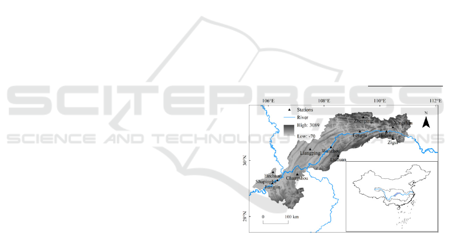
TGRA is located at the end of the upper reaches of
the Yangtze River (28°10'~31°50'N,
105°10'~110°50'E), with an area of approximately
81,000 square kilometers (Figure 1). Its topography
is characterized by deep valleys, rapid waters,
vertical and horizontal ravines, broken mountains,
frequent landslides, and a very fragile ecological
environment (Ma et al., 2015). The reservoir area
has a subtropical humid monsoon climate, with short
winters and long summers, with annual rainfall
ranging from 1000 to 1300 mm, abundant rainfall
but uneven seasonal distribution. TGRA has a
subtropical monsoon climate, and its annual average
temperature is 17
o
C. Affected by atmospheric
circulation and topography, the climate is unstable,
there are many types of disastrous weather, and the
frequency of floods and droughts is high, which
seriously harms agricultural production (Liu et al.,
2004).
2.2 Data Collection
This paper uses the daily data of 12 meteorological
stations (Xingshan, Badong, Zigui, Zhenping,
Fengjie, Wanzhou, Lichuan, Liangping, Changshou,
Shapingba, Jiangjin, Hechuan) from 1959 to 2019,
including the latitude and longitude of the stations,
the data for altitude, maximum temperature,
minimum temperature, average temperature,
sunshine hours, relative vapor pressure and 2m high
wind speed are all from the China Meteorological
Science Data Sharing Network (http://data.cma.cn/).
F
igure 1: The location of the reservoir area and the
distribution of meteorological stations.
3 METHODS
3.1 Penman-Monteith Method
This study is based on the Penman-Monteith method
(Li et al., 2016b) revised by the Food and
Agriculture Organization of the United Nations
(FAO) in 1998 to estimate the ET
0
corresponding to
the meteorological stations in TGRA. The
calculation formula is as follows:
Research on the Application of Non-stationary Model in Analyzing the Evolution Law of Reference Evapotranspiration
29

2
0
2
900
0.408 ( ) ( )
273
(1 0.34 )
nsa
R
Guee
T
ET
u
γ
γ
Δ−+ −
+
=
Δ+ +
(1)
Where,
Δ
is the slope of the saturated vapor
pressure curve (kPa
⋅
o
C
-1
), R
n
is the net solar
radiation(MJ
⋅
m
-2
⋅
d
-1
), G is the soil heat flux(MJ
⋅
m
-2
⋅
d
-1
),
γ
is the psychrometric constant (kPa
⋅
o
C
-1
),
U is the wind speed (m
⋅
s
-1
), T is the average
temperature (
o
C), e
s
is the average saturated vapor
pressure(kPa), e
a
is the actual vapor pressure(kPa).
The calculation process of R
n
, e
s
and e
a
is detailed in
literature (Bi et al., 2020).
3.2 Contribution Analysis based on
Sensitivity
The sensitivity coefficient is defined by the ratio of
ET
0
change rate to meteorological factor change rate,
which is used to quantify the contribution rate of
meteorological factors to ET
0
trend change (Zhang et
al., 2019). The multiplication of the sensitivity
coefficient of a single meteorological factor and its
multi-year relative change rate is the contribution
con(x) of the meteorological factor to the change of
ET
0
, and the contribution of each meteorological
factor is added to obtain the long-term trend of ET
0
.
In addition, the contribution rate of a single climate
factor to the long-term trend of ET
0
is p(x). If p(x) >
0, it means that the change of the factor has a
promoting effect on the change of ET
0
; if p(x) < 0, it
means that the change of the factor has an inhibitory
effect on the change of ET
0
.
00 0
0
0
/
lim ( )
/
x
x
ET ET ET
x
S
x
xxET
Δ→
Δ∂
==×
Δ∂
(2)
()
()
x
n slope x
con x S
x
⋅
=×
(3)
0
0
() ( ) ( ) ()
dET
con S con U con RH con T
ET
=+ + +
(4)
0
0
()
( ) 100%
con x
px
dET
ET
=×
(5)
Where, x is a meteorological factor, con(x) is the
contribution of a meteorological factor to ET
0
,
slope(x) is the tendency rate of x,
x
is the average
value of x in the period. x in this study refers to
sunshine hours (S), wind speed (U), relative
humidity (RH) and average temperature (T).
3.3 Generalized Additive Model based
on Location, Scale and Shape
Parameters
Generalized additive model based on location, scale,
and shape parameters (GAMLSS) is a (semi)
parametric regression model proposed by Rigby and
Stasinopoulos (Stasinopoulos et al., 2008) in 2005 to
analyze the non-stationary of series. It can flexibly
use multiple distributions to describe the
characteristics of random variable series, so as to
establish the linear or nonlinear relationship between
distribution parameters and covariates. Covariates
can be time or physical factors.
3.3.1 Model Definition
It is assumed that the observed value y
t
of random
variable at time t obeys the probability density
function
()
t
t
fy θ
, in which the distribution
parameter
t
θ can be reflected by the location
parameter (
1
θ
) and scale parameter (
2
θ
). The
mathematical description of the model is as follows:
1
()
k
J
kk k kk jkjk
j
gXZ θη
βγ
=
== +

(6)
Where,
k
η
is the observed value at time k, X
k
is an
explanatory variable matrix (which can be a time
series or a function of meteorological factors),
()
k
g ⋅
is a monotone differentiable connection function
(which represents the functional relationship
between
k
θ
and X
k
),
k
β
is the J
k
dimensional
regression parameter vector (which can be expressed
as
12
,,
k
T
kkkjk
βββ β = (, )
), Z
jk
and
j
k
γ
are the j-th
random effects.
Regardless of the influence of the random effect
term, and the random variable obeys a two-
parameter probability distribution, the general
expression of the GAMLSS model can be expressed
as:
11
()
g
X
μβ
=
(7)
22
()gX σ
β
=
(8)
The likelihood function of GAMLSS model with
regression parameter is as follows:
WRE 2021 - The International Conference on Water Resource and Environment
30

12 12
1
(, ) ( , )
n
t
t
Lfy
ββ ββ
=
=
∏
(9)
Taking the maximum value of the likelihood
function as the objective function, the RS algorithm
(Stasinopoulos et al., 2008) can be used to estimate
the optimal value of the regression parameters.
3.3.2 Model Construction
In this study, three models were constructed to
compare the evolution characteristics of ET
0
(Table
1). When the distribution parameters are constant, it
is the traditional stationary model (Model 0); When
at least one distribution parameter changes with time
t, it is a non-stationary model (Model 1). Model 1
has two fitting types, one is a linear function, the
other is a parabolic function, and the optimal
function fitting type is taken as the result of Model 1;
When at least one distribution parameter is
established as a function of meteorological factors, it
is a non-stationary model (Model 2).
Log normal distribution and gamma distribution
are selected to fit the annual maximum flow series of
each station in TGRA, and the AIC value of each
fitting is calculated. The smaller the AIC value is,
the better the corresponding model is. Therefore, the
annual maximum flow series is suitable for
stationary or non-stationary models. After selecting
the optimal fitting distribution by AIC value, the
model fitting is further judged by the distribution
characteristics of statistical model residuals.
2( ) #GAIC df θ =− + ⋅


(10)
Where, GAIC is the generalized AIC value,
() θ


is the log likelihood function corresponding to the
estimated values of regression parameters, df is the
degree of freedom of the model, # is the penalty
factor (When # = 2, GAIC is AIC value).
Table 1: Model distribution parameters and combination
of covariates.
Models Schemes
1
θ
or
2
θ
Model 0 1 ct
Model 1
2
01
t
ββ
+
3
2
01 2
tt
ββ β
++
Model 2
4
011
x
ββ
+
5
01122
x
x
ββ β
++
6
0112233
x
xx
ββ β β
++ +
4 RESULTS
4.1 Spatial Distribution Characteristics
of ET0
The multi-year average ET
0
of TGRA is between
743.9 and 1000.5 mm, with an average of 864.3 mm
(Figure 2e). From the upstream to the downstream of
the reservoir area, ET
0
first decreases and then
increases. The high-value areas are located in the
Daba Mountain, Wushan, and Yangtze River Valley
areas in the northeast of TGRA, and the low-value
areas are located on the south side of the upper and
middle reaches.
The four seasons and the annual ET
0
spatial
distribution are generally similar, and there is a
characteristic that high-value areas are located in the
lower reaches. The range of ET
0
in spring is
195.9~270.0mm, and the low value area is on the
south side of the middle and upper reaches (Figure
2a); the spatial range of ET
0
in summer is
307.1~396.8mm, and the low value area is in the
mountain area on the south side of the middle
reaches (Figure 2b); The range of ET
0
in autumn is
213.9~150.6mm, and the low-value area is in the
main urban area of Chongqing (Figure 2c); the
spatial range of ET
0
in winter is 75.3~132.3mm, and
the low-value area is in the Yangtze River Valley in
the middle reaches (Figure 2d). The order of the ET
0
value of each season is:
summer>spring>autumn>winter, accounting for
42%, 27%, 20%, and 11% of the annual value,
respectively. Among them, spring and summer
contribute the most to the annual value, nearly 69%.
Research on the Application of Non-stationary Model in Analyzing the Evolution Law of Reference Evapotranspiration
31

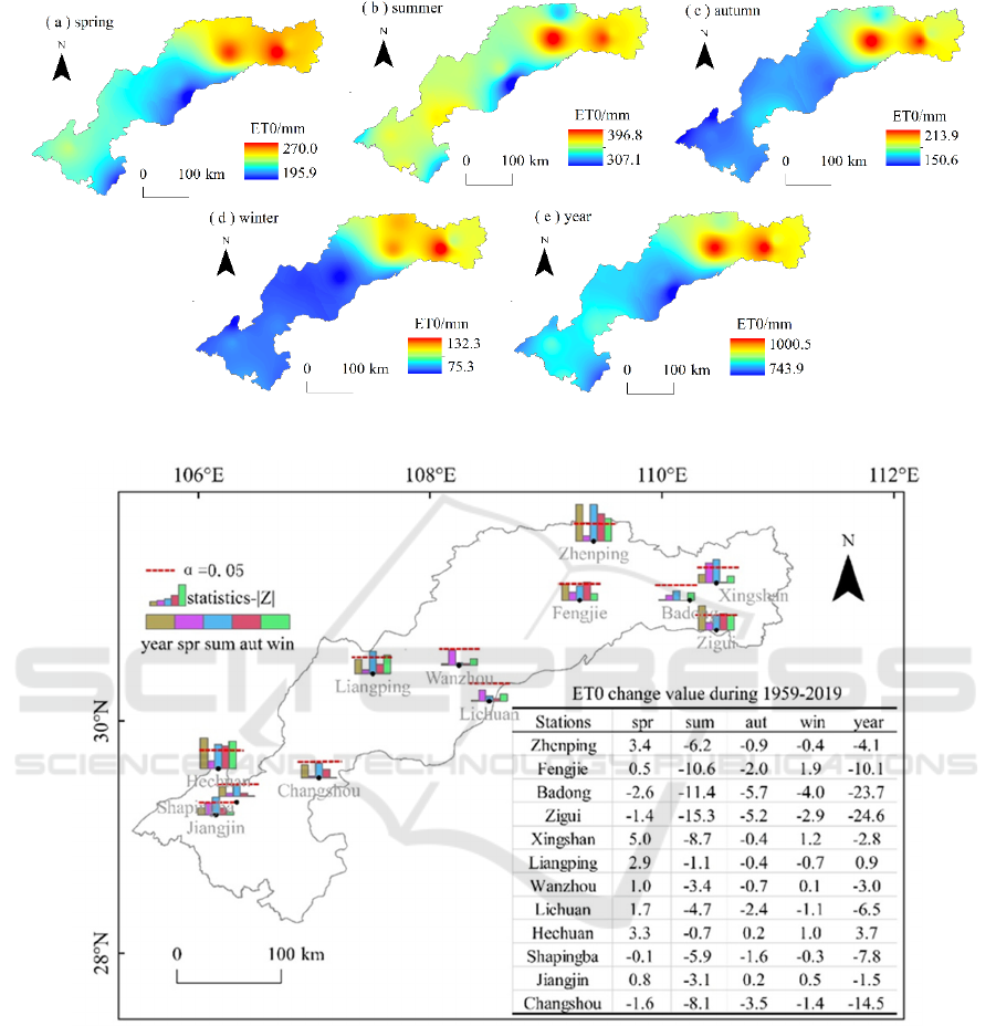
Figure 2: Spatial distribution of average ET0.
Figure 3: MK test and spatial distribution characteristics of change values of ET
0
(mm (10a)
-1
).
4.2 Seasonal Change Characteristics of
ET
0
The annual and seasonal ET
0
trend test and the
spatial distribution characteristics of the rate of
change of the 12 stations in TGRA (Figure 3). The
annual ET
0
has the Z value (MK's test statistics) of
ten twelfths stations are negative, the change value is
between -24.7~-1.5mm (10a)
-1
(P < 0.05). The
significant decrease in annual ET
0
was mainly
contributed by autumn and summer; the other two
stations showed an insignificant increase trend, and
the annual ET
0
change rate was 0.9 and 3.7mm
(10a)
-1
, respectively.
The ET
0
in the reservoir area showed an
insignificant increase trend in spring, a significant
decrease in summer ET
0
(P < 0.05), and an
insignificant decrease trend in the ET
0
series in
autumn and winter. The change rates of the four
seasons were 1.1, -6.6, -1.9, -0.5mm (10a)
-1
.
According to the pettitt mutation test, ET
0
mutation
occurred in 1979 in the year, summer and autumn
(Figure 4).
WRE 2021 - The International Conference on Water Resource and Environment
32

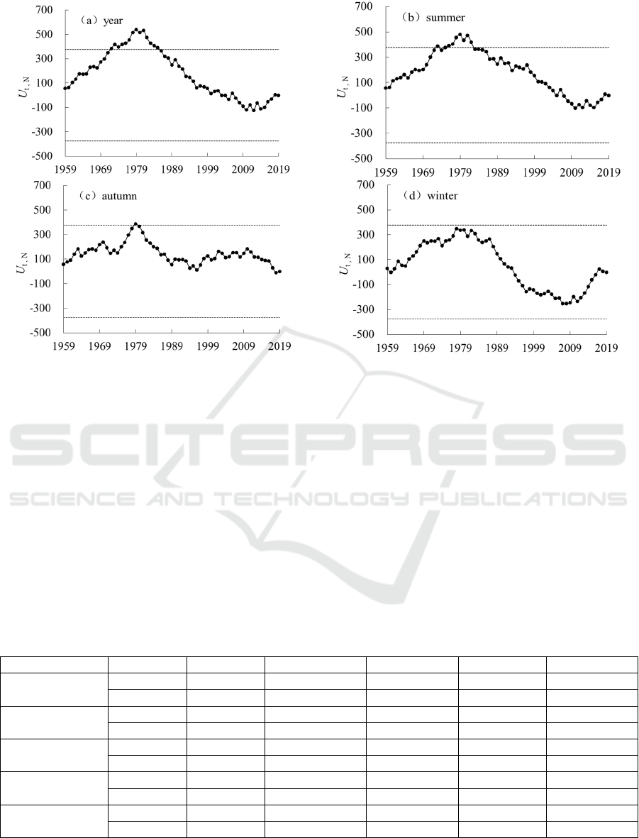
Figure 4: Annual and seasonal evaporation pettitt mutation test.
4.3 Driving Factor Analysis
Taking the seasonal mean values of S, U, RH, and T
of the 12 stations in TGRA as representative values,
the M-K test method is used to analyze the changing
trends of the main meteorological factors in the four
seasons, and the Z value of the statistics indicates a
significant trend. The k value represents the
tendency rate of the meteorological factor.
In the past 61 years, S, U, and RH in TGRA
showed a decreasing trend (Table 2). Since the mid-
1970s, the South Asian regional high and the
western Pacific subtropical high have tended to shift
to southwest China, and the East Asian monsoon has
a weakening trend, which is not conducive to the
production of wind and rain in southwest China
(Tabari et al., 2013), and T is also increasing year by
year, which has led to a downward trend in RH
during the past 61 years, and a significant downward
trend in U (P < 0.01 in spring, autumn and winter)
(Liu et al., 2018); Yang Xiaomei studied the S in
southwest China, which reveals that U is the main
reason for the changes in S. The significant increase
in T in TGRA (P < 0.05 in spring and autumn,
P<0.01 in winter) is mainly due to the impact of
global warming (Yang et al., 2012).
Table 2: M-K statistics and tendency rate of ET0 and meteorological factor.
Series Statistic S U RH T ET
0
Spring
Z 0.351 -4.742* -1.711 2.223** 0.572
k
0.001 -0.005 -0.035 0.012 0.107
Summer
Z -3.274* -2.161** 0.353 -0.192 -2.201**
k
-0.019 -0.002 0.003 -0.001 -0.660
Autumn
Z -2.562* -3.728* -0.486 2.138** -1.711
k
-0.009 -0.003 -0.005 0.011 -0.185
Winter
Z -1.213 -3.634* -0.525 2.616* -0.436
k
-0.006 -0.004 -0.010 0.016 -0.050
Year
Z -3.401* -4.031* -0.404 2.426** -2.262**
k
-0.008 -0.004 -0.013 0.009 -0.782
* indicate passing the 95% confidence test.
** indicate passing the 99% confidence test.
Research on the Application of Non-stationary Model in Analyzing the Evolution Law of Reference Evapotranspiration
33

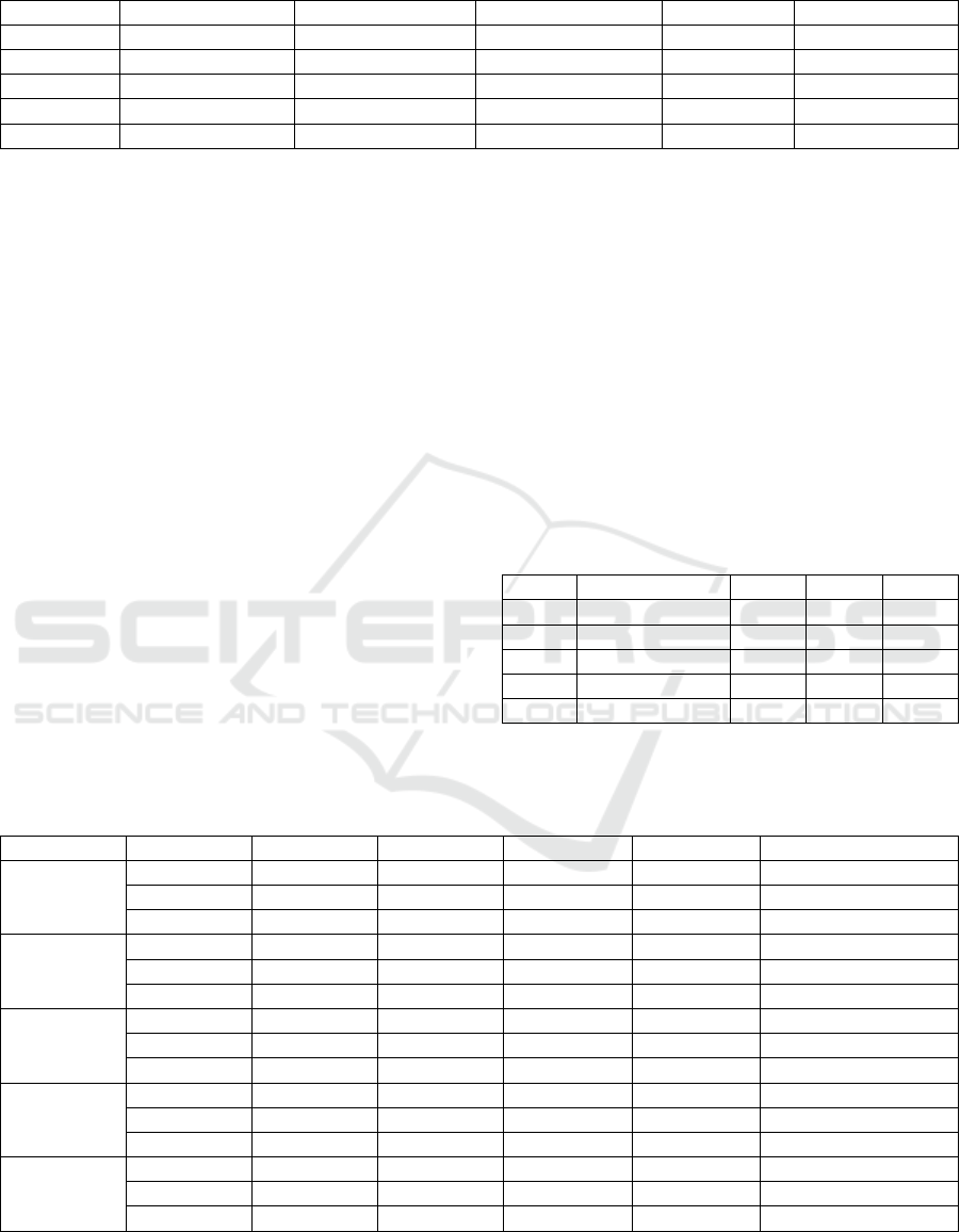
Table 3: Contribution rate of meteorological factors to ET0.
Series C(S) C(U) C(RH) C(T) C(ET
0
)
S
p
rin
g
62.01% -311.00% 297.06% 51.92% 100.00%
Summe
r
88.65% 9.84% 1.38% 0.13% 100.00%
Autumn 71.79% 41.79% -8.58% -5.00% 100.00%
Winte
r
66.02% 86.85% -30.91% -21.96% 100.00%
Yea
r
80.38% 48.32% -23.21% -5.48% 100.00%
Increasing (decreasing) of S, increasing
(decreasing) of U, decreasing (increasing) of RH,
and increasing (decreasing) of T will lead to an
increase (decrease) of ET
0
. The reason for the
significant decrease in annual ET
0
in TGRA is
caused by the combined effect of the decrease of S,
U, RH, and the increase of T. The contribution rates
of these factors are 80.38%, 48.32%, -23.21% and -
5.48%, respectively. Obtained that the promotion
effect of RH and T on ET
0
is less than the inhibitory
effect of S and U on ET
0
(Table 3). Summer ET
0
shows a significant decreasing trend. The
contribution rates of S, U, RH and T are 88.65%,
9.84%, 1.38% and 0.13%, respectively. The
decreasing of S, the increase of RH, the decrease of
temperature, and the decrease of wind speed all
contribute to ET
0
. Inhibition, so ET
0
showed a
significant decreasing trend (P < 0.05); spring,
autumn and winter will not be elaborated.
4.4 Non-stationary Evolution
The AIC criterion was used to analyze the fitting
results of Model 0, Model 1, and Model 2 (Table 4).
The best distribution of ET
0
in spring, autumn and
winter is the Gamma distribution, and the best
distribution of ET
0
in summer is the Normal
distribution. Model 1 has a smaller AIC value than
Model 0, that is, ET
0
in TGRA presents a non-
stationary evolution law with time as a covariate.
Compared with Model 0 and Model 1, when Model
2 uses meteorological factors as covariates to fit, the
reduction of AIC value is significantly improved,
indicating that the four seasons of the reservoir area
ET
0
series all show non-stationary with
meteorological factors as covariates. The following
takes the annual scale as an example to analyze the
inconsistent evolution law of the annual ET
0
.
Table 4: Comparison of AIC values between the stationary
model and the non-stationary model.
Series Best distribution Model 0 Model 1 Model 2
Spring GA 547.4 547.1 411.8
Summe
r
N
O 630.8 620.1 459.1
Autumn GA 515.8 515.3 436.4
Winte
r
GA 430.1 418.1 368.5
Yea
r
GA 668.1 654.5 593.9
GA—gamma distribution.
NO—normal distribution.
Table 5: Fitting residual distribution moments and Filliben coefficients of each model.
Series Models Mean Variance Skewness Kurtosis Filliben correlation
Spring
Model 0 0.00 1.0166 -0.0089 2.3731 0.9943
Model 1 0.00 1.0166 -0.0490 2.3483 0.9939
Model 2 0.00 1.0166 -0.0809 3.4609 0.9870
Summer
Model 0 0.00 1.0166 -0.0377 2.1356 0.9910
Model 1 0.00 1.0166 0.1415 2.1060 0.9890
Model 2 0.00 1.0166 0.2149 1.8555 0.9763
Autumn
Model 0 0.00 1.0166 0.2679 2.7754 0.9937
Model 1 0.00 1.0166 0.2045 3.0307 0.9925
Model 2 0.00 1.0166 -0.3125 3.1542 0.9913
Winter
Model 0 0.00 1.0166 0.2072 3.1358 0.9947
Model 1 0.00 1.0166 0.0378 2.4756 0.9935
Model 2 -0.01 1.0160 -0.0330 2.3311 0.9946
Year
Model 0 0.00 1.0166 0.0018 2.4222 0.9952
Model 1 0.00 1.0166 0.3001 2.8050 0.9934
Model 2 0.00 1.0166 0.2292 2.4102 0.9927
Quantile map of each model of annual ET
0
in
TGRA (Figure 5). The stationary model (Model 0)
cannot well capture the variation characteristics of
ET
0
scatter points (Figure 5a); the non-stationary
WRE 2021 - The International Conference on Water Resource and Environment
34

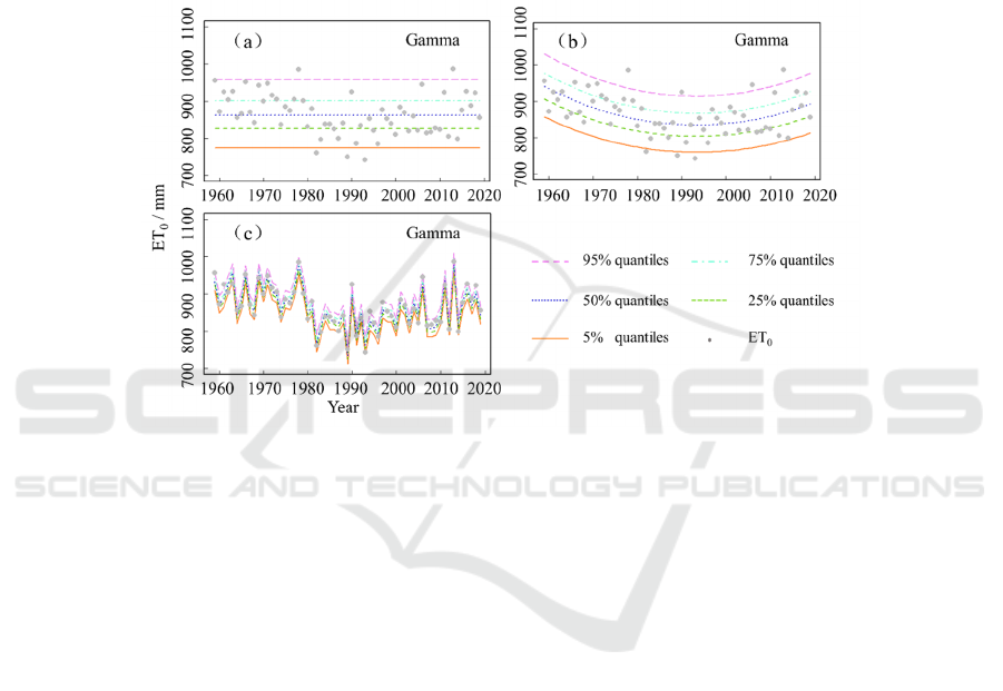
model (Model 1) with time t as a covariate can well
capture the time series distribution of ET
0
scatter
points (Figure 5b), ET
0
showed a downward trend
from 1959 to 1979, ET
0
showed an upward trend
from 1980 to 2019, and 1979 was a mutation point,
which is consistent with the results of the pettitt
mutation test. However, the Model 1 cannot
determine whether the annual ET
0
continues to
increase after 2019, and the fitting result lacks
physical meaning. The non-stationary model (Model
2) with meteorological factors as covariates captures
the ET
0
scatter better than Model 1, and the AIC
value is also significantly reduced, and has certain
physical meaning (Figure 5c). With meteorological
factors as the driving factor, the annual ET
0
dropped
sharply from 1978 to 1981, and then the ET
0
showed
an increasing trend in the following years.
The Filliben coefficients of the fitting residuals
of each model are basically greater than 0.979,
indicating that the residuals of each model obey the
normal distribution well (Table 5).
Figure 5: Comparison of quantiles diagrams between Model 0, Model 1 and Model 2.
5 CONCLUSIONS AND
SUGGESTIONS
In the past 61 years, the annual ET
0
of ten twelfths
stations has shown a decreasing trend by a linear
regression analysis, and the rate of decrease is -
24.7~-1.5mm (10a)
-1
. Among them, the annual ET
0
of Badong, Zigui and Changshou stations has
decreased significantly (p<0.05), the decrease is
mainly contributed by the autumn and summer
seasons. The annual and summer ET
0
decreased
significantly (p<0.05). There was a mutation in ET
0
in the year, summer and autumn in 1979.
The contribution rates of S, U, RH and T for the
significant decrease in annual ET
0
are 80.38%,
48.32%, -23.21% and -5.48% respectively, and the
promotion effect of RH and T on ET
0
is less than the
inhibitory effect of S and U on ET
0
.
The stationary model (Model 0) obviously cannot
explain the significant change trend and mutation
characteristics of ET
0
; the non-stationary model
(Model 1) with time as a covariate can capture that
the ET
0
sequence has a mutation in 1979, before and
after the mutation point ET
0
is a steep decrease and a
slow increase trend, respectively, explaining the
characteristics of the significant change trend and
sudden change of ET
0
, but lacks certain physical
meaning, and the future changes of ET
0
are difficult
to predict; a non- stationary model with
meteorological factors as covariates (Model 2) , It
can better capture the distribution of ET
0
scattered
points, and the AIC value is also significantly
reduced, verifying that the main contributing factors
that cause the annual ET
0
change are S, U, and RH,
which have certain physical significance.
ACKNOWLEDGMENTS
The researchers would like to extend theirs thanks to
the National Natural Science Foundation of China
(No. 51779271) and National Key Research and
Development Program of China (No.
2017YFC0404701).
Research on the Application of Non-stationary Model in Analyzing the Evolution Law of Reference Evapotranspiration
35

REFERENCES
Bi, Y. J., Zhao, J., Zhao, Y., Xiao, W. H., & Meng, F. J.
(2020). Spatial-temporal variation characteristics and
attribution analysis of potential evapotranspiration in
Beijing-Tianjin-Hebei region. Transactions of the
Chinese Society of Agricultural Engineering, 36(5),
130-140.
Han, H. Q., Bai, Y. M., & Zhang X. D. (2018). Study on
applicabilities and modifications of several methods
for estimating reference crop evapotranspiration in
Guizhou Province. Water Resources and Hydropower
Engineering, 49(10), 198-204.
Liu, C. Z., Li, T. F., Wen, M. S., Wang, X. P., & Yang, B.
(2004). Assessment and early warning on geo-
hazards in the Three Gorges Reservoir region of
Changjiang River. Hydrogeology & Engineering
Geology, 4(2), 9-19.
Liu, Y., Cui, N. B., Li, G., Luo, W. Q., Liao, G. L., &
Wang, L. T. (2018). Attribution Analysis of Seasonal
Reference Crop Evapotranspiration in Southwest
China in Recent 56 Years. Water Saving Irrigation,
280(12), 59-64.
Lu, F., Xiao, W. H., Yan, D. H., & Wang, H. (2017).
Progresses on statistical modeling of non-stationary
extreme sequences and its application in climate and
hydrological change. Journal of Hydraulic
Engineering, 48(4), 379-389.
Lu, F., Xiao, W. H., Dai, Y. Y., & Song, X. X. (2020a).
Research on non-stationary hydrological frequency
calculation in the mainstream of the Yellow River.
Journal of Hydroelectric Engineering, 221(12), 76-
84.
Lu, F., Song, X. Y., Xiao W. H., Zhu, K., & Xie, Z. B.
(2020b). Detecting the impact of climate and
reservoirs on extreme floods using nonstationary
frequency models. Stochastic environmental research
and risk assessment, 34(1), 169-182.
López, J., & Francés F. (2013). Non-stationary flood
frequency analysis in continental Spanish rivers,
using climate and reservoir indices as external
covariates. Hydrology & Earth System Sciences,
8(17), 3189-3203.
Li, S. E., Kang, S. Z., Zhang, L., Zhang, J. H., Du, T. S.,
& Tong, L. (2016a). Evaluation of six potential
evapotranspiration models for estimating crop
potential and actual evapotranspiration in arid
regions. Journal of Hydrology, 543, 450-461.
Li, Y. Z., Liang, K., Bai, P., Feng, A. Q., Liu, L. F., &
Dong, G. T. (2016b). The spatio-temporal variation
of reference evapotranspiration and the contribution
of its climatic factors in the Loess Plateau, China.
Environmental Earth Sciences, 75(4), 1-14.
Ma, J., Li, C. X., Wei, H., Ma, P., Yang, Y. J., Ren, Q. S.,
& Zhang, W. (2015). Dynamic evaluation of
ecological vulnerability in the Three Gorges
Reservoir Region in Chongqing Municipality, China.
Acta Ecologica Sinica, 35(21), 7117-7129.
Stasinopoulos, D. M., Rigby, R. A., & Akantziliotou, C.
(2008). Instructions on how to use the GAMLSS
package in R. Accompanying documentation in the
current GAMLSS help files.
Tabari, H., Grismer, M. E., & Trajkovic, S. (2013).
Comparative analysis of 31 reference
evapotranspiration methods under humid conditions.
Irrigation Science, 31(2), 107-117.
Xiong, L. H., Jiang, C., Du, T., Guo, S. L., & Xu, C. Y.
(2015). Review on Nonstationary Hydrological
Frequency Analysis under Changing Environments.
Journal of Water Resources Research, 4(4), 310-319.
Xing, Y., & He, Z. H. (2021). Study on Characteristics
and Driving Mechanism of Evapotranspiration of
Reference Crops in Vegetation Growing Season in
Karst Area, Taking Guizhou Province as an example.
Science Technology and Industry, 21(4), 264-272.
Yang, X. M., An, W. L., Zhang, W., Chang, L., & Wang,
Y. M. (2012). Variation of sunshine hours and related
forces in southwestern China. Journal of Lanzhou
University (Natural Sciences), 48(5), 52-59.
Zhang, D. D., Yan, D. H., Wang, Y. C., Lu, F., & Liu S.
H. (2015a). GAMLSS-based nonstationary modeling
of extreme precipitation in Beijing–Tianjin–Hebei
region of China. Natural Hazards, 77(2), 1037–1053.
Zhang, Q., Gu, X. H., Singh, V. P., Xiao, M. Z., & Chen,
X. H. (2015b). Evaluation of flood frequency under
non-stationarity resulting from climate indices and
reservoir indices in the East River basin, China.
Journal of Hydrology, 527, 565-575.
Zhang, P. F., Zhao, G. J., Mu, X. M., Gao, P., & Sun, W.
Y. (2019). Spatiotemporal Variation and Driving
Factors of Pan Evaporation in the Weihe River Basin.
Arid Zone Research, 36(4), 973-979.
WRE 2021 - The International Conference on Water Resource and Environment
36