Long-term Streamflow Forecasting and Uncertainty Analysis for

Hanjiang River using XGB Model

Huaping Huang

1,*

, Gaoyang Jin

1

, Kaixia Yin

1

, Ling Yi

1

, Dong Wang

2

and Yujie Li

3

1

China Water Resources Pearl River Planning Surveying & Designing Co., Ltd., Guangzhou 510610, China

2

Bureau of Hydrology, Changjiang Water Resources Commission, Wuhan 430010, China

3

Zhejiang Design Institute of Water Conservancy and Hydropower, Hangzhou 310002, China

Keywords: Long-term forecast, Monthly streamflow, Extreme gradient boosting, Model conditional processor,

Uncertainty analysis

Abstract: In this study, we proposed a hybrid modelling processor to generate highly performed streamflow forecasts.

As a demonstrated case, the extreme gradient boosting (XGB) algorithm was firstly employed to forecast

monthly streamflow series of the Huangzhuang hydrological station located in Hanjiang River Basin, China.

To further improve the forecast accuracy and quantify the uncertainty, model conditional processor (MCP)

approach was then used to postprocess the forecasts produced by the XGB model. The findings reveal that:

(1) the XGB algorithm performed well for simulating and forecasting monthly streamflow series, (2) The

median forecasts generated by the MCP approach exhibited smaller errors than the deterministic results of

XGB model. (3) The 90% confidence interval was reasonable and reliable as most of observations lied

within the prediction bounds.

1 INTRODUCTION

Over the past few decades, climate change and

human activities have intensified extreme

hydrological events such as frequent storm, flooding

and drought, which are often accompanied by the

life loss and damage to the infrastructures and the

environment (Hirabayashi et al., 2013). To solve this

problem, hydrologists and water resources

researchers have proposed many measures to

promote the disaster resilience and reduce losses.

Amongst, long-term streamflow forecasting exerts

an important effect in flood and drought control and

water resources system planning and management. It

has received tremendous attention of researchers due

to the resulting forecasts with a longer lead time,

which leaves enough time for effective responses

(Huang et al., 2019).

Various approaches have been proposed to

simulate and forecast the long-term streamflow series

based on either physical laws or system theoretic

approaches. The former approaches, such as

conceptual models or physically based models, were

designed to replicate the hydrological processes

(Devia et al., 2015). It is challenging to apply these

models for predicting long-term streamflow series as

they require complex mathematical tools, a large

amount of observed data and some practical

experience about the model. In recent years, with the

advance of artificial intelligence & data mining (AI

& DM) techniques, numerous machine learning

algorithms emerged and become more popular for

forecasting streamflow due to the advantage of

parsimonious data requirements and time-saving

procedures. Those AI & DM techniques, including

support vector machine (SVM), random forest (RF),

gradient boosting decision tree (GBDT), artificial

neural networks (ANN) and adaptive neuro-fuzzy

inference systems (ANFIS) have shown strong

abilities to produce reliable and accurate streamflow

forecasts (Yang et al., 2017, Ni et al., 2020, Pramanik

and Panda, 2009).

Although machine learning algorithms have been

widely applied for streamflow forecasting, few

studies assessed the uncertainties risen from the

input, model parameters and structures. The forecast

accuracy rapidly deteriorates as the lead time

increases, especially for long-term forecasting.

Therefore, it is important to identify and estimate the

uncertainties to ensure the resulting forecasts are

reasonable. Two primary approaches have been

developed for evaluating uncertainty, i.e., “error

Huang, H., Jin, G., Yin, K., Yi, L., Wang, D. and Li, Y.

Long-term Streamﬂow Forecasting and Uncertainty Analysis for Hanjiang River using XGB Model.

In Proceedings of the 7th International Conference on Water Resource and Environment (WRE 2021), pages 5-11

ISBN: 978-989-758-560-9; ISSN: 1755-1315

Copyright

c

5

analysis” methods or “element coupling” methods.

Error analysis methods directly estimate all

uncertainties in the forecasting process by

quantitatively establishing the relationship between

predictions and observations. Examples for such

methods include hydrologic uncertainty processor

(HUP) and model conditional processor (MCP)

(Krzysztofowicz and Herr 2001, Todini 2008). In

contrast, element coupling methods identify

different types of uncertainties associated with the

input data, model parameters and structures,

separately. Example for these methods include

rainfall calculation uncertainty (RCU), Bayesian

model averaging (BMA) and Bayesian total error

analysis (BATEA) (Hoeting et al., 1999, Kavetski et

al., 2006, Jiang 2019).

In this paper, we developed a hybrid modelling

processor by coupling the extreme gradient boosting

(XGB) algorithm and model conditional processor

(MCP) approach and applied it to the Hanjiang

River. The entire works entail: (1) selecting

predictors from numerous climate indices; (2)

generating deterministic forecasts using the XGB

model; (3) post-processing and assessing forecast

uncertainty using MCP approach. To test the model

performance, the deterministic result and the 90%

confidence interval were evaluated by different

performance indices.

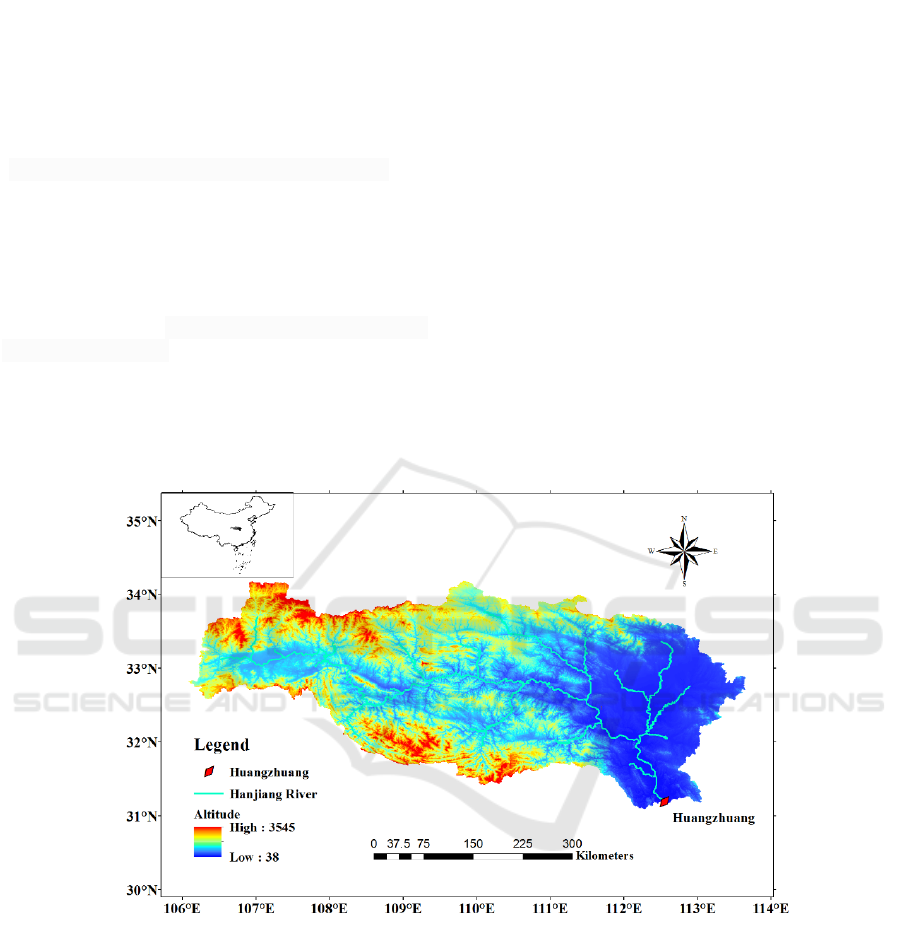
2 STUDY AREA AND DATA USED

The Hanjiang River is the longest tributary of the

Yangtze River and has a length of 1577 km and a

drainage area of 1.71 × 10

5

km

2

. This river

originates from Panzhong Mountain in Shanxi

Province and passes through Shanxi, Sichuan,

Henan and Hubei Provinces before entering the

Yangtze River in Wuhan. The characteristics of

Hanjiang River Basin and the location of

Huangzhuang station are shown in Figure 1.

Figure 1: The map of Hanjiang River Basin.

In this study, the monthly series from 1981 to

2017 of the Huangzhuang station located in the

Hanjiang River Basin were collected to calibrate and

validate the XGB model. A total of 130 climate

indices from 1980 to 2016 were obtained from the

China National climate Centre. Ten predictors for

each month were selected from all climate indices

for the last year through a correlation significance

test and a stepwise regression method. Selected

predictors for each month are not shown due to the

limited space of the paper.

3 METHODOLOGY

3.1 Extreme Gradient Boosting (XGB)

XGB, introduced by Chen & Guestrin (2016), is a

highly efficient boosting method based on the RF and

GBDT algorithm. As an improved version of

Gradient Boosting Machines, XGB has been

extensively employed to solve classification and

regression problems in many scientific fields, such as

WRE 2021 - The International Conference on Water Resource and Environment

6

bioinformatics, reservoir operation, remote sensing

and so on. This method fits the training data by using

an ensemble of classification and regression trees

(CART), each of which has an independent binary

tree decision rule structure. A more regularized

algorithm than gradient boosting is used to prevent

the regression model from overfitting data. In

addition, the computational time is minimized as

parallel calculations are automatically executed for

the objective functions in the training stage. Readers

are referred to Chen & Guestrin (2016) for more

details about the XGB model.

3.2 Model Conditional Processor

(MCP)

MCP is a conditional distribution-based method that

used for evaluating and reducing predictive

uncertainty. As an extended alternative of HUP, it

allows the estimation of density distribution of the

predictand conditional on all model forecasts at the

same time. The basic ideas of the MCP are

summarized as follows.

Step 1: The normal quantile transformation

(NQT) is used to transform observations

t

obs

Q

and

model forecasts

t

f

cst

Q

into normally distributed

variables separately.

()

t

t obs

NQT Q





;

()

t

tfcst

NQT Q







(1)

Step 2: The joint bivariate normal distribution

between transformed variables is built up, and the

parameters (the mean vector

,







, the covariance

matrix

,







) presented in Equation (2) need to be

estimated.





,

0, 0









;

1

,

1























(2)

Step 3: The density of predictand conditional on a

new forecast is derived based on the definition of the

bivariate normal distribution.

 

1/ 2

1

1/ 2 2

11

1

2exp(, ,)

11

2

(|)

(2 ) exp( / 2)

T

f

 





























(3)

Step 4: A huge number of samples can be

generated from the conditional distribution, and

back-transformation algorithm is used to convert the

samples into the real world.

1

()

mcp

QNQT







(4)

where

mcp

Q

is the final forecasting result,



is the

sample generated from conditional distribution.

3.3 Performance Indices

Performance indices, Nash-Sutcliffe efficiency index

(NSE), mean absolute percentage error (MAPE)

containing ration (CR), Average relative bandwidth

(RB) and average relative deviation amplitude (RD)

were used in this paper. Equations of these indices

can be found in Huang et al (2019).

4 RESULTS

4.1 Forecasting Results of XGB Model

The entire data set was divided into two parts,

including training set and validation set. The training

set was used to calibrate the XGB model, which

consisted of hydrological data from 1981 to 2007

and meteorological data from 1980 to 2006, and the

validation set was used to verify the calibrated

model, which consisted of hydrological data from

2008 to 2017 and meteorological data from 2007 to

2016. To avoid the problem of overfitting or

underfitting, the cross validation technique was

employed to calibrate the model in the training

period. The tree booster was used in this study, and

initial parameters was set as follows: eta=0.2,

max_depth=10, minimum_child_weigh=1,

subsample=0.95, alpha=0.3, gamma=1.The optimal

XGB model for each month was determined as the

one with the minimal MAPE value for the training

data throughout the cross validation, and the optimal

model was used to forecast the streamflow series for

the validation period.

Long-term Streamﬂow Forecasting and Uncertainty Analysis for Hanjiang River using XGB Model

7

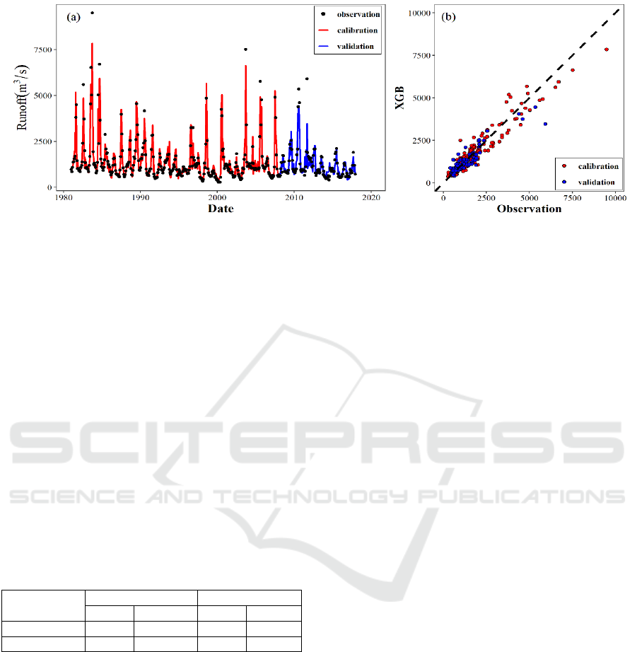
Figure 2: The observations and predictions from 1981 to 2017 for the XGB model.

The comparison and relationship between the

observed and predicted monthly streamflow series

for calibration and validation periods are shown in

the Figure 2. Predicted streamflow series of the

XGB model exhibit a good agreement with the

observed streamflow series, where the lower flow

points are dense and close to the diagonal line as

shown in the Figure 2(b). Compared with lower flow

points, higher flow points are more scattered and

more distant from the diagonal line. This finding

emphasizes the difficulty of predicting the extreme

values. Table 1 shows performance indices for the

results of the XGB model. The values of NSE and

MAPE are 0.91 and 15.3 in the training period, and

0.83 and 20.3 in the validation period, respectively,

reaffirming that the XGB algorithm is highly

effective for simulating and forecasting monthly

streamflow series of the Huangzhuang station.

Table 1: Performance indices of XGB and XGB-MCP.

Calibration Validation

NSE MAPE NSE MAPE

XGB 0.91 15.3 0.83 20.3

XGB-MCP 0.93 14.3 0.85 19.1

4.2 Postprocessing and Uncertainty

Analysis

To further enhance predictive accuracy and estimate

associated uncertainties quantitatively, the MCP

approach was employed to postprocess the

deterministic results from the XGB model. Again,

all data from 1981 to 2007 was used to train the

MCP model and estimate all parameters, and the

remaining data from 1981 to 2007 was used to

assess the model performance. The comparison

between the observations and ensemble forecast

medians was shown in Figure 3, and the

performance indices of ensemble forecast medians

were shown in Table 1.

Compared with the results in Figure 2, the points

in Figure 3(b) are closer to the diagonal line,

especially for the ones ranging from 4500 to 7000

m

3

/s. Referring to Table 1, the NSE and MAPE

values of XGB-MCP are larger and smaller than

those of XGB model for both training and validation

periods, respectively. It also indicates that the

ensemble forecast medians generated by the XGB-

MCP model are more accurate than the simulated

results from the XGB model. These findings suggest

that the MCP approach has a strong ability to

remove the bias and error associated with the

deterministic forecasts produced by the XGB model.

To investigate the reliability of the forecasts

generated by the MCP approach, the probability

integral transform (PIT) plots were used in this

paper, and the results are shown in Figure 4. All

points in Figure 4 are visually close to the diagonal

line and lie within the Kolmogorov 5% significance

bands. However, for the validation period, the points

are more distant away from the diagonal line than

those of calibration period. In Figure 4(b), the points

with uniform variate ranging from 0.125 to 0.35 are

distributed under the diagonal line, and the points

with uniform variate ranging from 0.7 to 0.85 are

above the diagonal line. This indicates that the

forecasts generated by the MCP approach is slightly

over-estimated compared with observations.

WRE 2021 - The International Conference on Water Resource and Environment

8

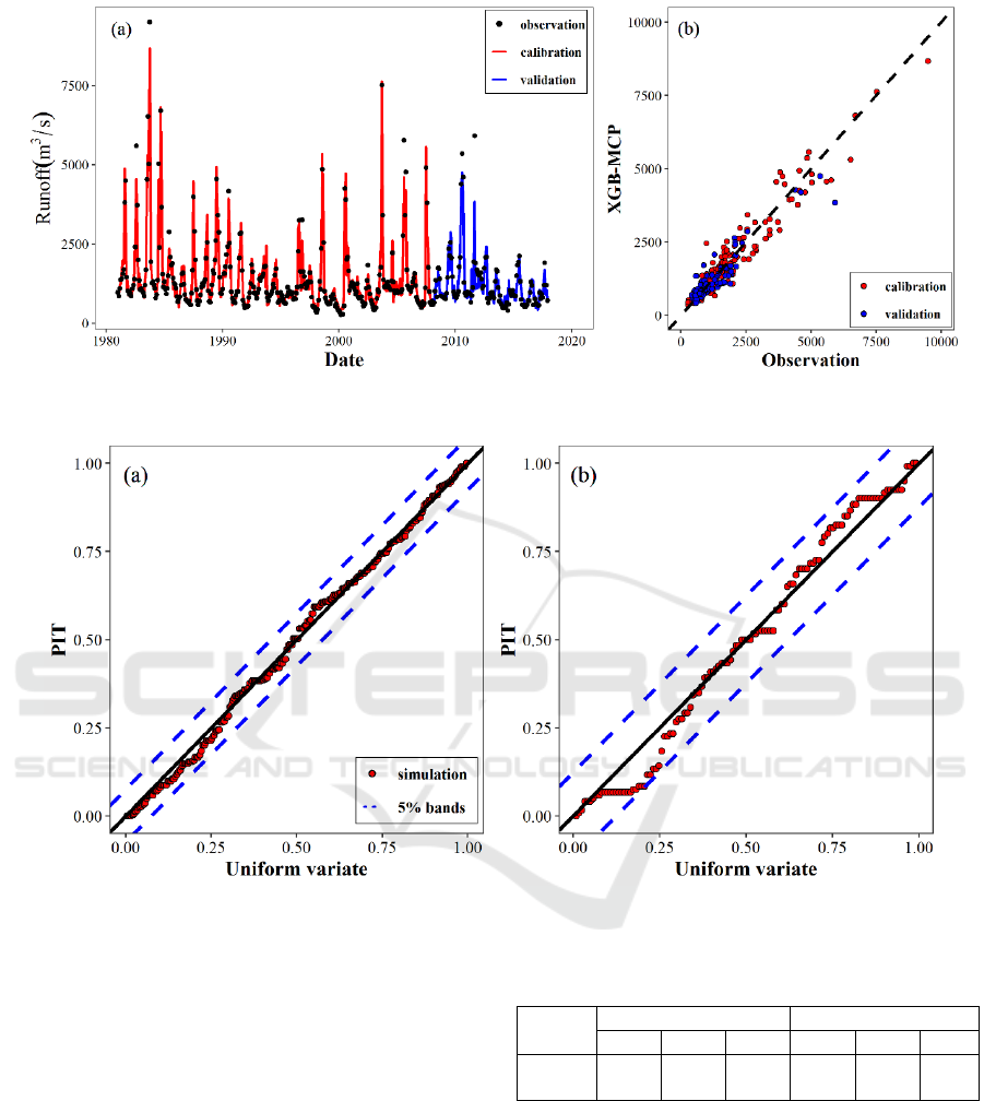
Figure 3: The observations and ensemble forecast medians from 1981 to 2017 for the XGB-MCP model.

Figure 4: PIT uniform probability plots for XGB-MCP model.

The 90% confidence intervals (90% CI) ranging

from 5% to 95% quantiles were also derived based

on the conditional distribution generated by the

MCP approach. Table 2 shows all performance

indices of the 90% confidence intervals for both

calibration and validation periods, and the 90%

confidence interval for validation period is presented

in Figure 5. It is found that more than 85% of

observations lies in the intervals with a relatively

narrow bandwidth, and the middle points between

prediction bounds are closer to the observations than

the results from the XGB model. All these findings

suggest that the 90% confidence intervals are

reasonable and reliable.

Table 2: Performance indices of 90% confidence intervals

generated by XGB-MCP model.

Calibration

V

alidation

CR RB RD CR RB RD

XGB-

MCP

0.93 0.65 0.15 0.85 0.67 0.20

Long-term Streamﬂow Forecasting and Uncertainty Analysis for Hanjiang River using XGB Model

9

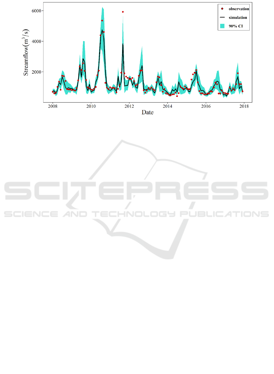
Figure 5: The 90% confidence interval of the XGB-MCP model for the validation period.

5 CONCLUSIONS

In this paper, the XGB model was employed to

simulate and predict monthly streamflow series of

the Huangzhuang station. To further enhance the

accuracy and eliminate uncertainties, the MCP

approach was used to postprocess the deterministic

results of the XGB model. The ensemble forecast

medians and 90% confidence intervals were

generated from the conditional distribution of the

predictand. Several performance indices were used

for evaluating the deterministic results and 90%

confidence intervals. Several conclusions can be

drawn as follows.

(1) The NSE and MAPE were selected as the

performance indices to investigate the accuracy

of the XGB model. Results reveal that it is

reasonable to apply the XGB model to predict

the monthly streamflow series of the

Huangzhuang station.

(2) Compared with results from the XGB model, the

NSE and MAPE values of the forecast medians

generated by MCP model were larger and

smaller, respectively, suggesting that the MCP

approach can remove the bias and error of the

forecasts generated by the XGB model.

(3) The CR, RB and RD indices were selected to

evaluate predictive uncertainties, the results of

which suggest that the 90% confidence intervals

cover most observations for both calibration and

validation periods, and the deviations of the

middle points from observed points are less than

0.2.

Although total predictive uncertainties in

hydrological process had been analysed and

estimated quantitatively in this study, we did not

distinguish uncertainties based on their sources, e.g.,

parameters, inputs and model structures. We also

ignored some other forecasting uncertainties risen

from external factors, including climate change and

human activities (Chen et al., 2011, Wesam et al.,

2020a, b). We will further investigate these

problems in the future work.

ACKNOWLEDGMENTS

This research has been financially supported by the

National Key Research and Development Program

of China (2018YFC1508200).

REFERENCES

Chen, T. and Guestrin, C. (2016). Xgboost: a scalable tree

boosting system. In: Proceedings of the 22nd ACM

Sigkdd International Conference on knowledge

Discovery and Data Mining (pp. 785-794). San

Francisco: ACM.

Chen, J., Brissette, F. P., Poulin, A., and Leconte, R.

(2011). Overall uncertainty study of the hydrological

impacts of climate change for a Canadian watershed.

Water Resources Research, 47(12), W12509.

Devia, G. K., Ganasri, B. P., and Dwarakish, G. S. (2015).

A review on hydrological models. Aquatic Procedia,

4, 1001-1007.

Hirabayashi, Y., Mahendran, R., Koirala, S., Konoshima,

L., Yamazaki, D., Watanabe, S., et al. (2013). Global

WRE 2021 - The International Conference on Water Resource and Environment

10

flood risk under climate change. Nature Climate

Change, 3(9), 816-821.

Hoeting, J. A., Madigan, D., Raftery, A. E., and Volinsky,

C. T. (1999). Bayesian Model Averaging: A Tutorial.

Statistical Science, 14(4), 382–401.

Huang, H., Liang, Z., Li, B., Wang, D., Hu, Y., and Li, Y.

(2019). Combination of multiple data-driven models

for long-term monthly runoff predictions based on

Bayesian model averaging. Water Resources

Management, 33(9), 3321-3338.

Jiang, X., Gupta, H. V., Liang, Z., and Li, B. (2019).

Toward improved probabilistic predictions for flood

forecasts generated using deterministic models. Water

Resources Research, 55(11), 9519-9543.

Kavetski, D., Kuczera, G., and Franks, S. W. (2006).

Bayesian analysis of input uncertainty in hydrological

modeling: 1. Theory. Water Resources Research, 42,

W03408.

Krzysztofowicz, R., and Herr, H. D. (2001). Hydrologic

uncertainty processor for probabilistic river stage

forecasting: precipitation‐dependent model. Journal of

Hydrology, 249(1–4), 46–68.

Ni, L., Wang, D., Wu, J., Wang, Y., Tao, Y., Zhang, J.,

and Liu, J. (2020). Streamflow forecasting using

extreme gradient boosting model coupled with

Gaussian mixture model. Journal of Hydrology, 586,

124901.

Pramanik, N., and Panda, R. K. (2009). Application of

neural network and adaptive neuro-fuzzy inference

systems for river flow prediction. Hydrological

Sciences Journal, 54(2), 247-260.

Todini, E. (2008). A model conditional processor to assess

predictive uncertainty in flood forecasting.

International Journal of River Basin Management,

6(2), 123–137.

Wesam, Mohammed-Ali., Cesar, Mendoza., Robert, R.,

and Holmes, Jr. (2020a). Influence of hydropower

outflow characteristics on riverbank stability: case of

the lower Osage River (Missouri, USA), Hydrological

Sciences Journal, 65(10), 1784-1793,

Wesam, Mohammed-Ali., Cesar, Mendoza., Robert, R.,

and Holmes, Jr. (2020b). Riverbank stability

assessment during hydro-peak flow events: the lower

Osage River case (Missouri, USA). International

Journal of River Basin Management, 19, 335-343.

Yang, T., Asanjan, A. A., Welles, E., Gao, X., Sorooshian,

S., and Liu, X. (2017). Developing reservoir monthly

inflow forecasts using artificial intelligence and

climate phenomenon information. Water Resources

Research, 53(4), 2786-2812.

Long-term Streamﬂow Forecasting and Uncertainty Analysis for Hanjiang River using XGB Model

11