Towards a Family of Digital Model/Shadow/Twin

Workﬂows and Architectures

Randy Paredis

1 a

, Cl

audio Gomes

2 b

and Hans Vangheluwe

1,3 c

University of Antwerp, Department of Computer Science, Middelheimlaan 1, Antwerp, Belgium

Aarhus University, DIGIT, Department of Electrical and Computer Engineering,

Abogade 34, Aarhus N, Denmark

Flanders Make@UAntwerp, Belgium

Keywords:

Digital Model, Digital Shadow, Digital Twin, Architecture, Workﬂow, Variability Modeling.

Abstract:

Digital Twins (DTs) can be used for optimization, analysis and adaptation of complex engineered systems,

in particular after these systems have been deployed. DTs make full use of both historical knowledge and of

streaming data from sensors. DTs have been given numerous (distinct) deﬁnitions and descriptions in the liter-

ature. There is no consensus on terminology, nor a comprehensive description of workﬂows nor architectures.

Following Multi-Paradigm Modelling principles, this paper proposes to explicitly model construction and use

workﬂows of DTs as well as their architectures. We apply the concepts of variability (also known as product

family) modeling, in particular to DT workﬂow and architecture. This allows for the de-/re-construction of the

different DT variants in a principled, reproducible and partially automatable manner. To illustrate our ideas,

two small use cases are discussed: a line-following robot (representative for an Automated Guided Vehicle)

and an incubator (representative for an Industrial Convection Oven). The use cases focus on important systems

in an industrial context.

1 INTRODUCTION

Digital Twins (DTs) are increasingly used Industry

4.0 and industrial processes for many purposes such

as monitoring, analysis, optimization. While their

deﬁnition has changed throughout the years, the con-

cept stayed somewhat the same: there exists a dig-

ital counterpart of a real-world system that provides

information about this system. Usually, this infor-

mation concerns itself with optimizations and correc-

tional behavior of this system.

Academic and industrial interest in DTs is grow-

ing, as they allow the acceleration through digitization

that is at the heart of Industry 4.0. Digital Twins are

made possible by technologies such as the Internet of

Things (IoT), Augmented Reality (AR), Product Life-

cycle Management (PLM) and many more.

Despite the many surveys on the topic (Rosen

et al., 2015; Negri et al., 2017; Kritzinger et al.,

2018; Cheng et al., 2018; Park et al., 2019; Zhang

et al., 2019; Aivaliotis et al., 2019; Kutin et al., 2019;

https://orcid.org/0000-0003-0069-1975

https://orcid.org/0000-0003-2692-9742

https://orcid.org/0000-0003-2079-6643

Bradac et al., 2019; Cimino et al., 2019; Lu et al.,

2020; Tao et al., 2019), there is no general consensus

on what characterizes a Digital Twin, let alone how it

is constructed. There is no one-deﬁnition-ﬁts-all and

therefore anyone in need of a DT starts from scratch to

build (what they believe to be) a DT. The main con-

cern is to create “value” for the user and to ensure

minimal re-use of workﬂows and architectures. To

some, a DT deﬁnes the virtual counterpart of the sys-

tem, while for others, it encompasses the full concept

of having both virtual and real systems at the same

time. For example, Lin and Low (2019) deﬁne DT

as “a virtual representation of the physical objects,

processes and real-time data involved throughout a

product life-cycle”, whereas Park et al. (2019) deﬁne

DT as “an ultra-realistic virtual counterpart of a real-

world object”.

This paper attempts to unify the most common

deﬁnitions and viewpoints in the form of a family of

problems solved by DTs as well as variant workﬂows

and architectures.

Several of the above cited surveys propose refer-

ence architectures for DTs. For instance, Bevilacqua

et al. (2020) proposes one that shares many common-

174

Paredis, R., Gomes, C. and Vangheluwe, H.

Towards a Family of Digital Model/Shadow/Twin Workﬂows and Architectures.

DOI: 10.5220/0010717600003062

In Proceedings of the 2nd International Conference on Innovative Intelligent Industrial Production and Logistics (IN4PL 2021), pages 174-182

ISBN: 978-989-758-535-7

alities with the other architectures. However, in a do-

main with so much variability for deﬁnitions and us-

age contexts, it is paramount that researchers apply

a systematic method to identify DT architectural pat-

terns.

Tekinerdogan and Verdouw (2020) have tried to

apply certain patterns to the design of DT and Gar-

nier et al. (2020) identiﬁes a set of patterns for a DT

architecture in a speciﬁc context. Their work provides

a basis which some of the ideas in this paper build on.

Van Acker et al. (2021) introduce the notion of valid-

ity frames to support precise reasoning about valid DT

contexts. In (Madni et al., 2019), four different lev-

els for modeling DTs were described. Note that the

patterns in the literature often mix problem domain,

architecture domain and deployment domain. In our

approach, we will separate and relate these.

This paper applies the variability modeling

methodology proposed in (Kang and Lee, 2013), to

systematically identify commonality and variability

in workﬂows and architectures for Digital Twins. In

order to illustrate our approach and make concepts

concrete, we apply our approach to the development

of Digital Twins for two complementary and small,

but representative, use cases. Our approach should be

generalizable towards larger systems.

The rest of this paper is structured as follows. Sec-

tion 2 discusses variability and product family model-

ing within the context of DT. Section 3 introduces two

simple use-cases that are representative for industrial

cases. Next, Section 4 discusses DT, starting from

variability modeling and presents a breakdown of a

DT architecture. Section 5 provides the workﬂow for

constructing DTs. Section 6 describes how engineer-

ing knowledge evolves over time and how this can be

captured in a Knowledge Graph. Finally, Section 7

concludes the paper.

2 VARIABILITY MODELING

It is common for multiple variants of a prod-

uct to exist. These variants share some common

parts/aspects/features/. . . but do vary in others. In the

automotive industry for example, it is common for ev-

ery sold car to be (often subtly) different due to small

differences in features. Such variants can often be

seen as different conﬁgurations.

To manage the often vast collection of variants,

the notion of a product family is used. Kang and Lee

(2013) separate the Variability Space in a Problem

Space and a Solution Space, as shown in Figure 1.

The variability in the Problem Space is broken down

into variability of User Goals and Objectives, Qual-

ity Attributes and the Usage Context of the products.

Variability in the Solution Space breaks down into

variability in the Capabilities, the Operating Environ-

ment and the Design of a solution to the problem. The

Capabilities deﬁne all different actors and their uses in

a system. Goals and Objectives drive the Capabilities

and Quality Attributes to be used in Quality Assur-

ance. The results applicable in the Solution Space can

be realized in an Artifact Space, that contains all ar-

chitectures, workﬂows, deployment options, modules

and components to be used in the realization (often

deployment in the context of software) of the solution

to the problem. As indicated by the “Drive”, “Mapped

To” and “Implemented By” arrows in the ﬁgure, there

is a natural ﬂow from a Real World Problem to a so-

lution, by making choices in each of the variability

sub-components. Based on these choices, the trans-

formations indicated by the arrows can be partially

automated. This ﬂow is called a (Software) Product

Line in the context of Generative Product Develop-

ment (Czarnecki et al., 2002).

Feature Modeling (Kang et al., 1990) is widely

accepted as a way to explicitly model variability.

One possible representation to capture variability in

a product family is by means of a Feature Tree (also

known as a Feature Model or Feature Diagram). It is

a hierarchical diagram that depicts the features that

characterize a product in groups of increasing lev-

els of detail. At each level, constraints in a Fea-

ture Tree model indicate which features are manda-

tory and which are optional. Traversing a Feature

Tree from its root downwards, features are selected

conforming to the constraints encode in the Feature

Tree model. This leads to a conﬁguration (feature se-

lection) which uniquely identiﬁes an element of the

product family. Note that Feature Trees are not the

only way to model product families. Wizards can

be used to traverse a decision tree and, in case the

variability is mostly structural, Domain-Speciﬁc Lan-

guages may be used (Czarnecki, 2004).

We propose to use Feature Models to capture the

variability in both the Problem Space and in the So-

lution Space. To illustrate our proposed approach, we

apply it to the two simple use cases of Section 3.

3 USE CASES

As this work is meant to guide the creation of DT in

a multitude of contexts, some exemplary use cases

are included to demonstrate the proposed architec-

tures (Section 4) and workﬂows (Section 5). A line-

following robot and an incubator use case are pre-

sented. These cases were chosen as representative

Towards a Family of Digital Model/Shadow/Twin Workﬂows and Architectures

175

Variability Space (Different Viewpoints)

Problem Space

Goal / Objective

Usage Context

Quality Assurance

Solution Space

Capability

Operating

Environment

Design Feature

Real World

Problem

Artifact Space

Product Line Asset

Subsystem

Architecture

Process

Architecture

Deployment

Architecture

Module Architecture

and Components

Space

Variability

Category

Drive

Mapped To

Implemented By

Figure 1: Variability Modeling Space (Kang and Lee, 2013).

(exhibiting the essential complexity) for their indus-

trial counterparts: an automated guided vehicle and

an industrial oven, respectively.

3.1 Line-following Robot

A simple transportation device in an industrial set-

ting is an Automated Guided Vehicle (AGV). This

is a computer-steered vehicle that allows the trans-

portation of materials, resources and people. For the

purposes of this use case, a Line-Following Robot

(LFR) is used as a simpliﬁcation of an AGV. The LFR

drives over a surface that contains a line (which can

be painted, reﬂective, ﬂuorescent, magnetized, . . . ),

with the sole purpose of following that line as closely

as possible. However, unexpected situations (e.g., the

robot cannot ﬁnd the line anymore, a forklift is block-

ing the robot’s trajectory, . . . ) are difﬁcult to all ac-

commodate for during the (LFR controller) design

phase. Uncertainty about unforeseen changes in the

LFR’s environment are one of the scenarios where a

Digital Twin provides a solution.

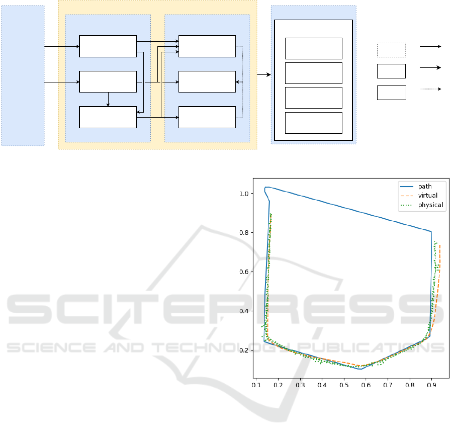
The proposed architecture and workﬂow have

been applied to construct a Digital Shadow (DS) (see

Section 4.1) for the LFR, which is described in de-

tail in (Paredis and Vangheluwe, 2021). The robot

drives on a predeﬁned surface. Its position is objec-

tively measured by a depth vision camera, mounted

statically above the surface at a height to allow the

camera’s ﬁeld of view to capture the entire driving

range. In Figure 2, trajectory data for this system

are presented. The blue, full line represents the the

line to follow, the orange, striped line identiﬁes the

DS’s simulation results and the green, dotted line rep-

resents the Physical Object’s identiﬁed position.

Figure 2: Example experiment results for the LFR.

3.2 Incubator

A heating chamber (i.e., an industrial oven) is com-

monly used in industry for curing, drying, baking, re-

ﬂow,. . . It introduces high-temperature processes to

the creation of a product. Some ovens allow this prod-

uct to be transported through the heating chamber on

a conveyor belt (or even an AGV).

The temperature in an industrial oven needs to be

regulated, as a change in temperature could damage

the product. For instance, glazed ceramics could have

a completely different color when baked at the wrong

temperature. Additionally, such a system has to re-

act to unpredictable changes in its environment (e.g.,

complete a safety shutdown when a person enters the

chamber during the baking process). This makes an

industrial oven an excellent example for the use of a

DT.

IN4PL 2021 - 2nd International Conference on Innovative Intelligent Industrial Production and Logistics

176

Similar to the previous use case, a simpliﬁcation

of such a device is made for the purposes of this paper,

to focus on the essential DT workﬂows and architec-

tures. An incubator is a device that is able to maintain

a speciﬁc (variable) temperature within an insulated

container. When the temperature is in the right range,

a baking process can be performed.

The incubator consists of ﬁve main components:

an thermally insulated container, a heatbed (for rais-

ing the temperature), a fan (for circulating the airﬂow,

which, through air convention, allows a uniformly

distributed temperature when in steady-state), three

temperature sensors (two are used to measure the in-

ternal heat, one is used for the temperature outside

the container – the environment, which is outside our

control) and a controller. This controller is similar to

a bang-bang (or on/off ) controller, but it has to wait

after each actuation, to ensure that the temperature is

raised gradually.

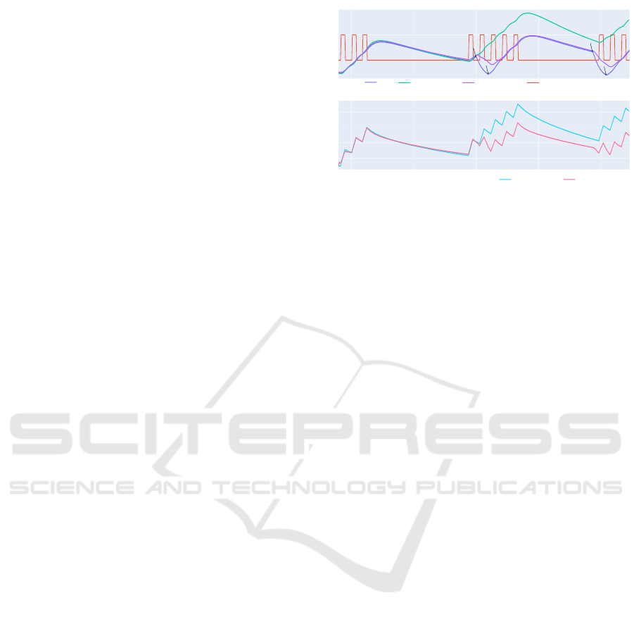
As with the LFR, this case was used to investi-

gate DT architecture and workﬂow. In (Feng et al.,

2021), a full description of this incubator is given.

Figure 3, adapted from (Feng et al., 2021), shows

an example where the lid of the incubator is opened

and that is detected as an anomaly by a Kalman ﬁlter

(Kalman, 1960) (purple temperature trajectory is the

Kalman ﬁlter; the blue trajectory is the real tempera-

ture as measured inside the incubator.). The Kalman

ﬁlter uses a model for the prediction of the tempera-

ture. Such a model does not consider the dynamics

of the temperature when the lid is open. As a result,

when the lid is opened, the predictions start to per-

form poorly, a fact that can be leveraged to perform

anomaly detection. Note that the ﬁgure also shows a

simulation that runs completely independently of the

measured data. The reason the Kalman ﬁlter does

not perform as poorly as this simulation is because

it still takes into account real sensor data. This, in

contrast to the simulation, which uses a model of the

environment. Also note that, compared to the simula-

tion, after the lid is closed, the simulation has a harder

time returning to normal, whereas the Kalman ﬁlter,

because it uses the measured data, quickly returns to

tracking the system behavior.

4 DIGITAL TWINS

The concept of the Digital Twin dates back to a Uni-

versity of Michigan presentation to industry in 2002

(Grieves and Vickers, 2017). Since its origin, the con-

cept has changed such that many research groups and

companies introduced their own deﬁnition(s), despite

many surveys on the topic.

14:50

Jan 22, 2021

14:55 15:00 15:05 15:10

avg_T

heater_onavg_temp(4pModel) avg_temp(Kalman)

T_heater(4pModel) T_heater(Kalman)

Incubator Temperature

Heat-bed Temperature

Timestamp

Lid Opened

Lid Closed

Lid Opened

Lid Closed

Figure 3: Example experiment where an anomaly is de-

tected using the Kalman ﬁlter. Adapted from (Feng et al.,

2021).

There is, however, a consensus on the goals and

objectives a DT can accomplish. Visualization, safety

monitoring and analysis, predictive maintenance,

fault tolerance, self-adaptation, self-reconﬁguration

and many more analysis-oriented concepts can be

solved using DTs. What is important is that the use of

DTs usually concerns complex systems with a certain

level of uncertainty due to limited knowledge about

the environment (e.g., human interaction).

This leads to the main challenges of this work (and

DT research in general): how can a DT be systemati-

cally engineered such that variability is allowed, qual-

ity ensured and the real-world problem solved?

4.1 DT Variability

Based on our experience with the two use cases and

on the extensive DT literature, we built feature models

for each of the blocks in Figure 1. Note that these are

by no means complete, but rather meant as a starting

point to illustrate our approach.

A (sub)set of the most common Goals for a DT

is shown in Figure 4. Notice the separation of the

mandatory “Observe” and the optional “Observe and

Modify”. This separation identiﬁes the split between

analysis, whereby the real-world system is not modi-

ﬁed, and adaptation, where it is.

The Usage Context for a DT is shown in the fea-

ture model of Figure 5. In the ﬁrst layer under Usage

Context, all features are mandatory. There is always

some User, always a Scale, always a Product Life-

cycle Stage, . . . This is an indication that these are or-

thogonal dimensions. Feature choices in each of these

dimensions can be combined. The context in which

the DT is active will constrain downstream choices

in the Solution Space. Figure 6 shows a selection of

Quality features. As with the Usage Context, in the

ﬁrst layer under Quality, all features are orthogonal

Towards a Family of Digital Model/Shadow/Twin Workﬂows and Architectures

177

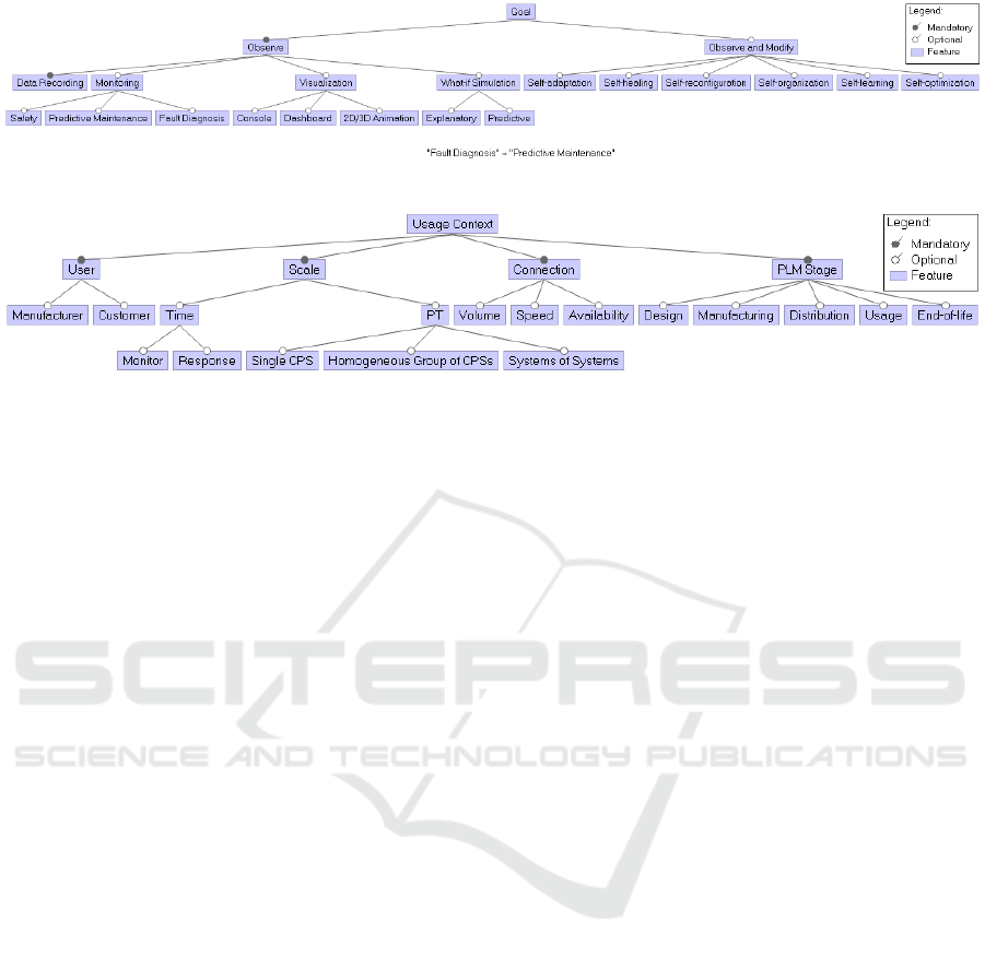
Figure 4: Feature model of the goals of a DT.

Figure 5: Feature model of the usage contexts of a DT.

and hence mandatory. The ﬁrst example dimension

concerns the quality of the various data connections

in the DT architecture. What these connections are

depends on the chosen architecture. The second ex-

ample dimension concerns the Ilities. According to

(de Weck et al., 2011), the Ilities are desired proper-

ties of systems, such as ﬂexibility or maintainability

(usually but not always ending in “ility”), that often

manifest themselves after a system has been put to

its initial use. These properties are not the primary

functional requirements of a system’s performance,

but typically concern wider system impacts with re-

spect to time and stakeholders than are embodied in

those primary functional requirements. The Ilities do

not include factors that are always present.

4.2 DT Design Variants

For the Solution Space, we currently do not use Fea-

ture Trees. Rather, in Figure 7, we show the three

main DT Design variants (Kritzinger et al., 2018).

As shown in Figure 7, each variant contains a Phys-

ical Object (PO) and a Digital Object (DO). The PO

represents the System under Study (SuS) within its

Environment. The DO represents a virtual copy of

the SuS (often in the form of a real-time simulator),

trying to mimic its behavior, assuming it is active

in the exact same Environment as the PO. Depend-

ing on one’s viewpoint and the application domain,

“physical” may be an ambiguous term as not all SuS

are constructed from what we typically call physical

(mechanical, hydraulic, . . . ) components. The SuS

may also contain software components. Furthermore,

imagine a (ﬁctional) 3D virtual world in which a SuS

exists for which a DT needs to be built. The SuS is

not physical in this example; hence, the more gen-

eral term “Realized Object” (RO) is proposed. Alter-

natively, the same logic can be applied on the DO.

For instance, a DO of a train may be modeled using

a scale model of the train, instead of a simulation. In

this case, the DO will be an “Analog Object” (AO) or

Analog Twin instead. For the purpose of this paper,

the focus will be on DOs.

The three main Design variants of DTs follow

from the nature of the data/information ﬂow between

RO and DO. In a Digital Model (DM), there is no au-

tomated ﬂow of data/information between the objects.

The only way data/information is transferred is by a

human user. If something changes in the RO, the DO

must manually be updated to conform to the new RO,

and vice-versa.

In a Digital Shadow (DS) however, the data ﬂow

from the RO to the DO becomes automated (i.e., with-

out human intervention). This data, more speciﬁ-

cally, is environmental information captured by sen-

sors. This, to ensure that the RO and the DO “see”

the same Environment. This is an important step, as it

allows a precise analysis of the accuracy and validity

of both objects. In Figure 4, the Observe family of

goals will lead to a DS solution.

Finally, the Digital Twin (DT) closes the loop be-

tween RO and DO. If something now changes in the

DO, the RO will receive an automated update corre-

sponding to this change. This is usually optimiza-

tion information, fault tolerance notiﬁcation, predic-

tive maintenance instructions, etc. Note that in the

DT case, automation may also refer to the inferenc-

ing and decision making without human intervention.

When building a DT, these variants are typically

all traversed in different “stages” in the creation pro-

cess. When a system exists as a DM, the introduc-

tion of an appropriate data communication connection

yields a DS. When the DO of a DS is now expanded

to do system analysis and optimizations (and the RO

IN4PL 2021 - 2nd International Conference on Innovative Intelligent Industrial Production and Logistics

178

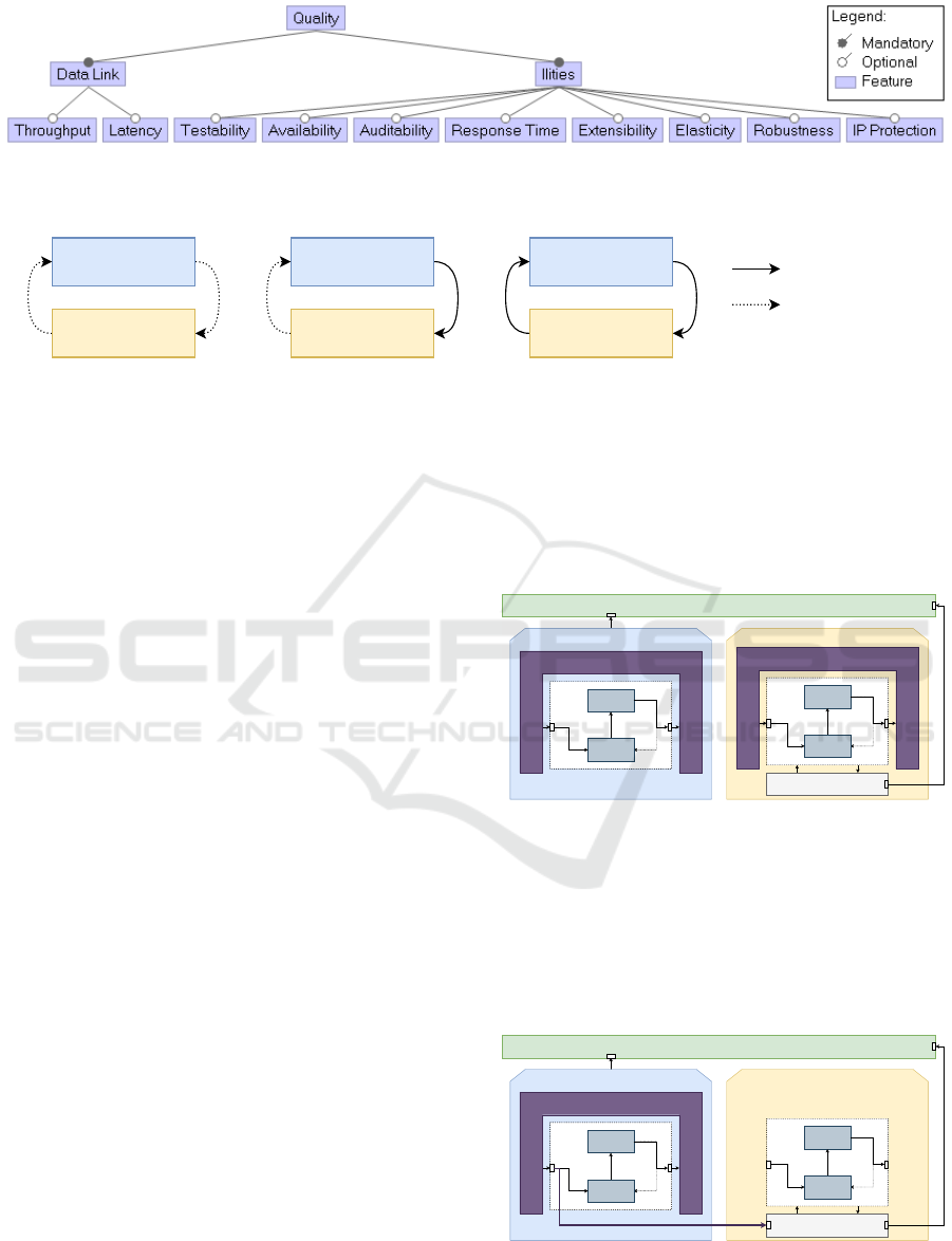
Figure 6: Feature model of the quality assurance of a DT.

Realized / Physical

Object

Digital

Object

Digital Model

Realized / Physical

Object

Digital

Object

Digital Shadow

Realized / Physical

Object

Digital

Object

Digital Twin

Automatic Data Flow

Manual Data Flow

Figure 7: Three main Design variants of DTs.

is able to evolve to allow for system adaptation), we

obtain a DT. Note that there needs to be an initial plan

to build a DT, so the architecture of the RO can be en-

gineered to allow for adaptation. If there was no origi-

nal plan to build a DT, modifying an existing RO may

be hard. Making the RO conﬁgurable from the out-

side as an afterthought may introduce security risks.

Figure 7 gives a high-level view on a DM/DS/DT.

Technically, this can be expanded by introducing an

External Object (EO). The EO implements one or

multiple external processes that require information

from or need to send data to the RO and the DO.

The purpose may be visualization, predictive mainte-

nance, analysis, optimization,. . . Whereas, originally,

these processes were typically part of the DO, the sys-

tem breakdown becomes much more streamlined by

logically including them in the EO. The EO’s func-

tionality may still, at deployment time, be included in

the DO. The EO almost always contains an observa-

tion “harness” that allows the objective (independent

from the DO) collection of data from the RO and its

environment. In the LFR, this is an H-bar on which a

depth-vision camera is mounted, supplemented with

a Kalman ﬁlter for a moving window estimator of the

RO’s state (position and heading). For the incuba-

tor, this harness only consists of the sensors that were

used. In (Paredis and Vangheluwe, 2021), this harness

is called the “External System Analyzer” (ESA).

In Figure 8, a high-level architecture is shown for

the DM. The SuS is modeled as a Plant-Controller

model (the faint, dotted arrow identiﬁes an optional

feed-back loop). Both in the RO and in the DO, this

SuS interacts with an Environment. For the DO, how-

ever, this Environment is a modeled mock-up of the

real environment. It should interact with the SuS in

exactly the same way as the real environment. In

practice, the environment will model a typical “duty

cycle” of the SuS. The DO also includes a Real-Time

Simulator used to simulate the SuS and Environment

models.

Every component of this ﬁgure is implemented

with the techniques and technologies that best match

the selected Goals, Usage contexts and Quality re-

quirements of the system.

DIGITAL OBJECT

REAL-TIME SIM

SuS

model

PLANT

CTRL

VIRTUAL MOCK-UP ENV

REALIZED OBJECT

SuS

PLANT

CTRL

ENVIRONMENT

EXTERNAL OBJECT

Figure 8: High-level DM architecture.

When taking a closer look at Figure 9, a high-level

architecture for a DS, it becomes clear that (in the

DO) the mock-up Environment is now replaced by a

data connection from the input of the SuS in the RO.

This provides both RO and DO sub-systems with the

exact same input and should, therefore, yield identical

behavior in both.

DIGITAL OBJECT

REAL-TIME SIM

SuS

model

PLANT

CTRL

REALIZED OBJECT

SuS

PLANT

CTRL

ENVIRONMENT

EXTERNAL OBJECT

Figure 9: High-level DS architecture.

Towards a Family of Digital Model/Shadow/Twin Workﬂows and Architectures

179

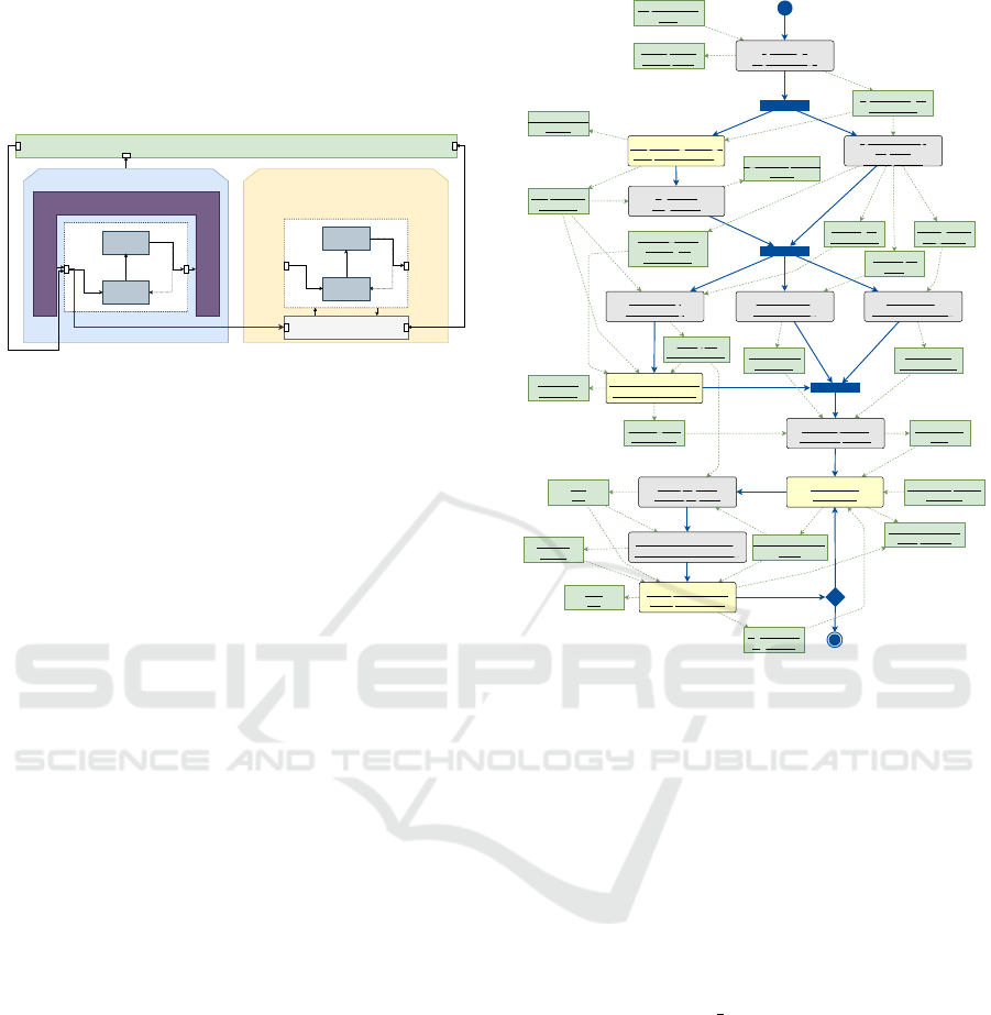
Figure 10 shows a similar architecture for a DT.

Compared to the DS, a connection from the EO goes

towards the inputs of both SuS. If the EO identiﬁes

the need for a change in the RO, it will ask the SuSs

in both RO and DE to apply this change.

DIGITAL OBJECT

REAL-TIME SIM

SuS

model

PLANT

CTRL

REALIZED OBJECT

SuS

PLANT

CTRL

ENVIRONMENT

EXTERNAL OBJECT

Figure 10: High-level DT architecture.

Multiple technologies exist to deploy communica-

tion links. RabbitMQ (https://www.rabbitmq.com/),

Ditto (https://www.eclipse.org/ditto/), RTI (https://

www.rti.com/), to name a few. Depending on the se-

lected Goals and Quality requirements of the system,

a speciﬁc technology can be chosen.

Notice how Figures 8, 9 and 10 describe variant

architectures. They are models in an appropriate Ar-

chitecture Domain-Speciﬁc Language (DSL). DSLs

are more appropriate than Feature Trees when the

variability is structural.

Finally, a “Digital X” (where X stands for Model,

Shadow, or Twin) is a System in its own right,

which means that all Model-Based System Engineer-

ing (MSBE) techniques can, and should, be used to

design it. Conversely, DTs can be used as components

in a system. Each DT component corresponds to a

particular aspect of interest of the system. Note that

this recursive combination of the specialization and

containment relationships implies higher-order DTs.

5 WORKFLOW

The previous section presented the general architec-

ture of DMs/DSs/DTs. In addition to architectures

and their deployment, the worﬂow describes in which

order which activities are carried out, on which ar-

tifacts. A well-chosen workﬂow may optimize the

overall development process time. A workﬂow or

Process Model (PM) follows partly from the con-

straints imposed by the variability models and their

relationships (Drives, Mapped To, Implemented By)

in Figure 1. Figure 11 shows a PM that yields a

DT with an architecture described in Figure 10. It

has been created by analyzing and unifying the work-

ﬂows followed for both cases from Section 3. The

requirements :

SRS

sys_design

: System Design

assumptions :

Assumptions

component_gathering :

ComponentGathering

bill_of_material

: BOM

components :

Hardware

digitization

: Digitization

digital_components

: CAD

system_decomp

: System

Decomposition

eo_design : 2D

Drawings +

Architecture

ro_design :

Architecture

System Design :

Architecture

harness_construction :

HarnessConstruction

ro_assembly

: ROAssembly

prototype :

ROAssembled

plant_modeling

: PlantModeling

ctrl_modeling

: ControllerModeling

plant_eqs :

ODE

ctrl_algorithm

: Algorithm

harness :

Hardware

param_guess

: Constants

sus_composition

: SuSComposition

plant_model :

PlantDSL

ctrl_model :

ControllerDSL

sus_model :

DSL

virt_mockup_env :

Emulator

calibration :

Calibration

ro_deployment

: RODeployment

tuned_sus_model

: DSL

communication_modeling

: CommunicationModeling

ro :

server :

Server

eo_implementation :

EOImplementation

eo :

digital_twin :

DigitalTwin

simulation_results

: Plot, Table...

Figure 11: Workﬂow model for the construction of a DT.

PM shown is modelled as a UML Activity Diagram,

describing the order of activities (control ﬂow), an-

notated with their in- and output artifacts (data ﬂow).

The roundtangles represent the activities carried out

and the rectangles identify the input/output artifacts.

All activities and artifacts have a name and a type,

denoted as “name : Type”. Some of the activi-

ties can be automated. This depends on the mod-

eling languages and tools that were used. Yellow

roundtangles represent hierarchical activities, indi-

cating that they encapsulate a sub-workﬂow. For

instance, “component gathering” could entail col-

lecting all necessary components from a set of usable

parts (e.g., the LFR was built using the LEGO Mind-

storms EV3 Core Set (313131)) or it could consist of

deﬁning the component requirements and buying the

corresponding parts (as was the case for the incuba-

tor).

In the following, we detail some of the process

steps. The “digitization” activity may be skipped

if there is no need for the CAD models of the system.

Alternatively, this can be done after the DT has been

constructed.

For all DT systems, an external (to the RO) set of

sensors is required to obtain the true current state of

the SuS. This is called the DM/DS/DT “harness”. For

IN4PL 2021 - 2nd International Conference on Innovative Intelligent Industrial Production and Logistics

180

the incubator, this consists of the temperature sensors.

The LFR, however, requires an H-bar construction, on

which a depth-camera is mounted. When constructing

this harness (the “harness construction” activity),

a set of benchmark tests is performed to help in the

calibration of the harness, but also to yield an initial

guess for the parameters of the system, which will be

altered by the “calibration” activity. This activity

uses a “virt mockup env” (called the “emulator” in

(Feng et al., 2021)) in which the DO runs. This is

a virtual abstraction of the environment that interacts

with the DO, just like the RO interacts with the real

environment (see Figure 8). This yields a DM that

allows testing and continuous integration of the DT

before it is connected to the real system. Once an ac-

ceptable result is obtained, the RO is deployed and a

communication link established between the DO and

the RO. Real-world experiments may provide new in-

sights that cause the “calibration” activity to be en-

tered again.

6 KNOWLEDGE EVOLUTION

One may wonder where the knowledge used to con-

struct a DM/DS/DT comes from. This knowledge,

when explicitly represented, takes the form models

in various formalisms, including historical data from

earlier experiments. We use a Knowledge Graph

(KG) to store this knowledge (and made available

in a KG server). The KG is used in the design of

a DM/DS/DT Experiment, by means of the variabil-

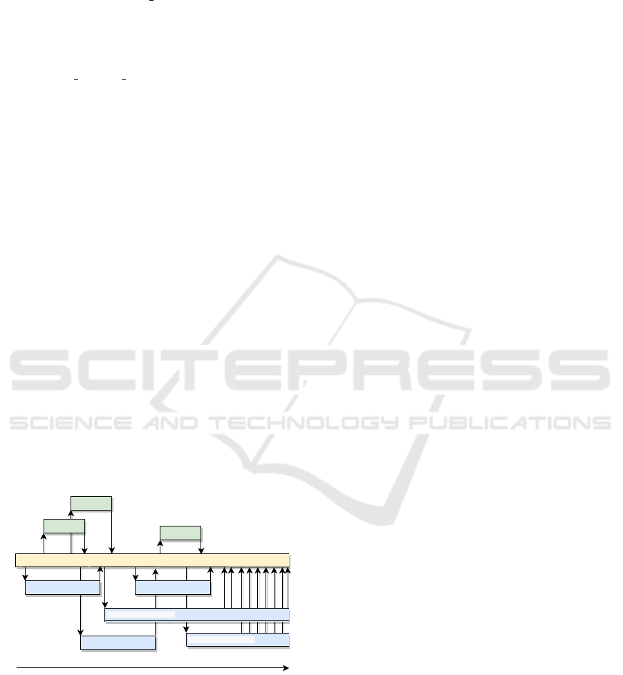
ity models and workﬂow described earlier. Figure 12

shows an example of the interaction between the KG

Knowledge Graph

time

DM/DS/DT Experiment 1

DM/DS/DT Experiment 3

DM/DS/DT Experiment 4

Inferencing

DM/DS/DT Experiment 2

DM/DS/DT Experiment 5

Figure 12: KG and DM/DS/DT Experiment Interaction.

(server) and DM/DS/DT experiments. Given a partic-

ular user question Q, the data/information/knowledge

in the KG is used to design a DM/DS/DT experiment

architecture that, when deployed as experiment E, can

provide an answer A to the question. The DM/DT/DS

may use historical information and/or it may interact

in real-time with real-world physical assets. Exper-

iments 1, 2 and 3 in the ﬁgure are bounded in time

(also known as terminating). When they ﬁnish, their

results (i.e., the triple (Q, E, A) is stored in the KG.

Long-running “streaming” experiments 4 and 5 will

store intermediate, partial answers in the KG. Ex-

periment 5 stores periodically, whereas Experiment 4

does so when deemed relevant (e.g., whenever suf-

ﬁcient new information has become available). It is

noticed that many experiments can be performed in

parallel. When setting up an experiment to answer

a question, all information available in Knowledge

Graph at that time, included that which was added

by earlier experiments, can be used. Asynchronous

inferencing may also update the KG, by for example

turning data into information into knowledge.

7 CONCLUSIONS

This paper has presented an architecture and a

workﬂow for creating (a family of) Digital Mod-

els/Shadows/Twins using Multi-Paradigm Modelling

principles (Amrani et al., 2021). The feasibility of

the approach has been demonstrated by means of

two distinct use cases (which may be combined in

an industrial setting) that are simpliﬁcations of of-

ten used industrial components. A Knowledge Graph

has been introduced as a knowledge repository from

which an experiment is constructed to answer ques-

tions. This DM/DS/DT experiment then provides an

answer to the question, which get added to the Knowl-

edge Graph. We plan to further explore the various

product family models introduced here. More impor-

tantly, the relationships between the features will be

further investigated, with as ultimate goal, to auto-

mate as much as possible of the workﬂow.

ACKNOWLEDGEMENTS

This research was partially supported by Flanders

Make, the strategic research centre for the Flem-

ish manufacturing industry and by a doctoral fellow-

ship of the Faculty of Science of the University of

Antwerp. In addition, we are grateful to the Poul Due

Jensen Foundation, which has supported the estab-

lishment of a new Centre for Digital Twin Technology

at Aarhus University.

Towards a Family of Digital Model/Shadow/Twin Workﬂows and Architectures

181

REFERENCES

Aivaliotis, P., Georgoulias, K., and Alexopoulos, K. (2019).

Using digital twin for maintenance applications in

manufacturing: State of the Art and Gap analysis. In

2019 IEEE International Conference on Engineering,

Technology and Innovation (ICE/ITMC), pages 1–5,

Valbonne Sophia-Antipolis, France. IEEE.

Amrani, M., Blouin, D., Heinrich, R., Rensink, A.,

Vangheluwe, H., and Wortmann, A. (2021). Multi-

paradigm modelling for cyber–physical systems: a de-

scriptive framework. Software and Systems Modeling.

Bevilacqua, M., Bottani, E., Ciarapica, F. E., Costantino,

F., Donato, L. D., Ferraro, A., Mazzuto, G., Monteri

A., Nardini, G., Ortenzi, M., Paroncini, M., Pirozzi,

M., Prist, M., Quatrini, E., Tronci, M., and Vignali, G.

(2020). Digital twin reference model development to

prevent operators’ risk in process plants. Sustainabil-

ity (Switzerland), 12(3).

Bradac, Z., Marcon, P., Zezulka, F., Arm, J., and Benesl,

T. (2019). Digital Twin and AAS in the Industry 4.0

Framework. IOP Conference Series: Materials Sci-

ence and Engineering, 618:012001.

Cheng, Y., Zhang, Y., Ji, P., Xu, W., Zhou, Z., and Tao, F.

(2018). Cyber-physical integration for moving digi-

tal factories forward towards smart manufacturing: A

survey. The International Journal of Advanced Man-

ufacturing Technology, 97(1-4):1209–1221.

Cimino, C., Negri, E., and Fumagalli, L. (2019). Review of

digital twin applications in manufacturing. Computers

in Industry, 113:103130.

Czarnecki, K. (2004). Overview of generative software de-

velopment. In Ban

atre, J., Fradet, P., Giavitto, J.,

and Michel, O., editors, Unconventional Program-

ming Paradigms, International Workshop UPP, Re-

vised Selected and Invited Papers, volume 3566 of

LNCS, pages 326–341. Springer.

Czarnecki, K., Østerbye, K., and V

olter, M. (2002). Gener-

ative programming. In N

nez, J. H. and Moreira, A.

M. D., editors, Object-Oriented Technology, ECOOP

2002 Workshops and Posters, volume 2548 of LNCS,

pages 15–29. Springer.

de Weck, O. L., Roos, D., Magee, C. L., and Vest, C. M.

(2011). Life-Cycle Properties of Engineering Systems:

The Ilities, pages 65–96. MIT Press.

Feng, H., Gomes, C. a., Thule, C., Lausdahl, K., Iosiﬁdis,

A., and Larsen, P. G. (2021). Introduction To Digi-

tal Twin Engineering. In 2021 Annual Modeling and

Simulation Conference (ANNSIM).

Garnier, J.-L., Bachatene, H., and Nowodzienski, P. (2020).

Architecture Patterns for Digital Twins in Space Ap-

plications. Presentation at the AFNeT Standard-

ization Days: https://download.afnet.fr/ASD2020/

ASD2020-13a-DigitalTwin-JeanLucGarnier.pdf, ac-

cessed: 2021-05-28.

Grieves, M. and Vickers, J. (2017). Digital Twin: Mitigat-

ing Unpredictable, Undesirable Emergent Behavior in

Complex Systems. In Transdisciplinary Perspectives

on Complex Systems, pages 85–113. Springer.

Kalman, R. E. (1960). A New Approach to Linear Filtering

and Prediction Problems. Journal of Basic Engineer-

ing, 82(1):35–45.

Kang, K. and Lee, H. (2013). Variability Modeling. In

Systems Software and Variability Management, pages

25–42.

Kang, K. C., Cohen, S. G., Hess, J. A., Novak, W. E.,

and Peterson, A. S. (1990). Feature-oriented domain

analysis (FODA) feasibility study. Technical report,

Carnegie-Mellon University.

Kritzinger, W., Karner, M., Traar, G., Henjes, J., and Sihn,

W. (2018). Digital Twin in manufacturing: A cat-

egorical literature review and classiﬁcation. IFAC-

PapersOnLine, 51(11):1016–1022.

Kutin, A. A., Bushuev, V. V., and Molodtsov, V. V. (2019).

Digital twins of mechatronic machine tools for mod-

ern manufacturing. IOP Conference Series: Materials

Science and Engineering, 568:012070.

Lin, W. D. and Low, M. Y. H. (2019). Concept and imple-

mentation of a cyber-physical digital twin for a SMT

line. In 2019 IEEE International Conference on In-

dustrial Engineering and Engineering Management

(IEEM), pages 1455–1459.

Lu, Y., Liu, C., Wang, K. I.-K., Huang, H., and Xu,

X. (2020). Digital Twin-driven smart manufactur-

ing: Connotation, reference model, applications and

research issues. Robotics and Computer-Integrated

Manufacturing, 61:101837.

Madni, A. M., Madni, C. C., and Lucero, S. D. (2019).

Leveraging Digital Twin Technology in Model-Based

Systems Engineering. Systems, 7(1):7.

Negri, E., Fumagalli, L., and Macchi, M. (2017). A Review

of the Roles of Digital Twin in CPS-based Production

Systems. Procedia Manufacturing, 11:939–948.

Paredis, R. and Vangheluwe, H. (2021). Exploring A Dig-

ital Shadow Design Workﬂow By Means Of A Line

Following Robot Use-Case. In 2021 Annual Model-

ing and Simulation Conference (ANNSIM).

Park, H., Easwaran, A., and Andalam, S. (2019). Chal-

lenges in Digital Twin Development for Cyber-

Physical Production Systems. In Chamberlain, R.,

Taha, W., and T

orngren, M., editors, Cyber Physical

Systems. Model-Based Design, volume 11615, pages

28–48. Springer International Publishing, Cham.

Rosen, R., von Wichert, G., Lo, G., and Bettenhausen, K. D.

(2015). About The Importance of Autonomy and Dig-

ital Twins for the Future of Manufacturing. IFAC-

PapersOnLine, 48(3):567–572.

Tao, F., Zhang, H., Liu, A., and Nee, A. Y. C. (2019). Digi-

tal Twin in Industry: State-of-the-Art. IEEE Transac-

tions on Industrial Informatics, 15(4):2405–2415.

Tekinerdogan, B. and Verdouw, C. (2020). Systems Archi-

tecture Design Pattern Catalog for Developing Digital

Twins. Sensors, 8(18):5103.

Van Acker, B., Mertens, J., De Meulenaere, J., and De-

nil, J. (2021). Validity Frame Supported Digital

Twin Design of Complex Cyber-Physical Systems. In

2021 Annual Modeling and Simulation Conference

(ANNSIM).

Zhang, H., Ma, L., Sun, J., Lin, H., and Th

urer, M. (2019).

Digital Twin in Services and Industrial Product Ser-

vice Systems:. Procedia CIRP, 83:57–60.

IN4PL 2021 - 2nd International Conference on Innovative Intelligent Industrial Production and Logistics

182