Anomaly Detection in Multivariate Spatial Time Series: A Ready-to-Use

Implementation

Chiara Bachechi

, Federica Rollo

, Laura Po

and Fabio Quattrini

“Enzo Ferrari” Engineering Department, University of Modena and Reggio Emilia, Italy

Keywords:

Anomaly Detection, Spatial Time Series, Spatio-temporal Data, IoT, Sensor Network.

Abstract:

IoT technologies together with AI, and edge computing will drive the evolution of Smart Cities. IoT devices

are being exponentially adopted in the urban context to implement real-time monitoring of environmental

variables or city services such as air quality, parking slots, trafﬁc lights, trafﬁc ﬂows, public transports etc. IoT

observations are usually associated with a speciﬁc location and time slot, therefore they are spatio-temporal

collections of data. And, since IoT devices are generally low-cost and low-maintenance, their data can be

affected by noise and errors. For this reason, there is an urgent need for anomaly detection techniques that are

able to recognize errors and noise on sensors’ data streams. The Spatio-Temporal Behavioral Density-Based

Clustering of Applications with Noise (ST-BDBCAN) algorithm combined with Spatio-Temporal Behavioral

Outlier Factor (ST-BOF) employs both spatial and temporal dimensions to evaluate the distance between

sensor observations and detect anomalies in spatial time series. In this paper, a Python implementation of

ST-BOF and ST-BDBCAN in the context of IoT sensor networks is described. The implemented solution has

been tested on the trafﬁc ﬂow data stream of the city of Modena. Four experiments with different parameters’

settings are compared to highlight the versatility of the proposed implementation in detecting sensor fault and

recognizing also unusual trafﬁc conditions.

1 INTRODUCTION

Modern smart cities employ numerous sensors to

monitor several aspects of city life, i.e. vehicular traf-

ﬁc, parking availability, air quality, and others. The

huge amount of data streams produced by sensor net-

works needs data cleaning processes to detect outliers

and remove unreliable data before further analysis.

Indeed, anomaly detection is one of the most impor-

tant challenges in data mining. In an urban sensor

network, the comparison of data coming from close

sensors (neighborhood information) can be exploited

to improve the identiﬁcation of anomalies. Trafﬁc

sensors are an example of faulty sensors. Anoma-

lies in trafﬁc sensor observations can heavily affect

the results of the subsequent analysis, such as trafﬁc

ﬂow simulation, trafﬁc trend analysis, trafﬁc monitor-

ing, and prediction. Trafﬁc sensor observations can

be seen as a time series (considering only one sen-

sor at a time) or as a spatial time series (consider-

ing more than one sensor and their relative position).

https://orcid.org/0000-0003-2323-0573

https://orcid.org/0000-0002-3834-3629

https://orcid.org/0000-0002-3345-176X

Trafﬁc sensors are usually ﬁxed; hence, each sensor

generates a geolocated time series associated with its

position. Exploiting spatial information for anomaly

detection makes the approach more robust because it

allows not only to compare a sensor’s measurements

with respect to its past measurements but also to the

measurements of close sensors. On the other hand,

managing the spatial features is very challenging.

Spatio-temporal outlier detection is the identiﬁcation

of objects that exhibit abnormal behavior either spa-

tially, and/or temporally. Even if there is an ur-

gent need for algorithms that classify outliers based

on space and time features, there are not many al-

gorithms of this type in literature. Mainly, meth-

ods are divided between algorithms for the identiﬁ-

cation of outliers based on the temporal component

(Wang et al., 2019a; Gupta et al., 2014) and algo-

rithms that are based on the spatial component (such

as Local Outlier Factor (LOF) (Breunig et al., 2000),

DBSCAN (Ester et al., 1996) and the merge of the

two: LDBSCAN (Duan et al., 2007)). For detect-

ing spatio-temporal outliers using both the spatial and

temporal features, a promising approach has been re-

cently published, combining the Spatio-Temporal Be-

Bachechi, C., Rollo, F., Po, L. and Quattrini, F.

Anomaly Detection in Multivariate Spatial Time Series: A Ready-to-Use Implementation.

DOI: 10.5220/0010715900003058

In Proceedings of the 17th International Conference on Web Information Systems and Technologies (WEBIST 2021), pages 509-517

ISBN: 978-989-758-536-4; ISSN: 2184-3252

509

havioral Outlier Factor (ST-BOF) in cascade with the

Spatio-Temporal Behavioral Density-based Cluster-

ing of Applications with Noise (ST-BDBCAN) (Dug-

gimpudi et al., 2019) algorithm. ST-BDBCAN is

based on the distinction between spatio-temporal and

behavioral attributes. Spatio-temporal attributes in-

dicate the position of the sensors or provide tempo-

ral information about the observation. Behavioral at-

tributes instead are all the other attributes that refer to

the given spatio-temporal point, i.e. measured values,

environment variables. ST-BDBCAN groups objects

with similar behavioral attributes as clusters and de-

tects objects with abnormal behavioral attributes as

outliers, exploiting the outlier factors evaluated by

ST-BOF. To the best of our knowledge, there is no

code implementation of these two algorithms avail-

able online.

In this paper, we focused on the study of ST-BOF

and ST-BDBCAN and produced its implementation

in Python (the code is available online

with exemplar

data to execute the algorithm). The proposed imple-

mentation is realized for multivariate spatial time se-

ries but can be easily adapted to spatio-temporal time

series (where both spatial and temporal dimensions

vary for each observation). The proposed implemen-

tation is suitable for the application of the algorithm

to different contexts. In this paper, we discuss the ap-

plication of the algorithm to data collected by 49 traf-

ﬁc sensors in the city of Modena, in Italy.

Several

experiments have been conducted with different con-

ﬁguration parameters of ST-BOF and ST-BDBCAN

in order to investigate the difference in the types of

anomalies detected.

The paper is organized as follows. Section 2 dis-

cusses related work on anomaly detection in spatial

time series. In Section 3, a brief explanation of ST-

BOF and ST-BDBCAN is given, and we focus on

describing the characteristic of our implementation.

Then, Section 4 is devoted to the description of our

use case, while Section 5 presents in detail four ex-

periments and compares their results. Section 6 is

dedicated to conclusions.

2 RELATED WORK

Several techniques have been developed to identify

anomalies in spatio-temporal data. In recent years,

https://github.com/quattrinifabio/ST-BOF

ST-BDBCAN

Hourly sensor trafﬁc data are published as Open

Data on the Emilia Romagna Open Data portal (Desi-

moni et al., 2020) at https://dati.emilia-romagna.it/dataset/

hourly\\-trafﬁc-observation-linked-data-2018-2020.

also Machine Learning based anomaly detection ap-

proaches have been successful. In (Rollo et al., 2021)

the authors selected 12 unsupervised anomaly detec-

tion algorithms, such as Angle-base Outlier Detec-

tion, Isolation Forest, clustering-based Local Outlier,

and trained them on air quality sensor data to iden-

tify and remove abnormal data patterns. Anomaly

detection techniques can be divided into two main

categories: distance-based and clustering-based. In

distance-based techniques, the spatio-temporal dis-

tance between instances is evaluated with different

approaches and then the instances whose distance

from the other instances is above an established

threshold are considered as outliers. Among distance-

based algorithms, an interesting solution is proposed

by (Bachechi et al., 2020; Bachechi et al., 2021)

that describes a novel data cleaning process to de-

tect anomalies in real-time trafﬁc data streams. The

proposed methodology exploits the Seasonal-Trend

Decomposition using Loess (STL) and the study of

the Interquartile Range on the remainder component

of the time series. Distance-based anomaly detec-

tion methods could not handle datasets with different

density areas effectively. For this reason, clustering-

based approaches can be an interesting alternative

since the identiﬁcation of outliers is based on density:

the instances in regions with low density are labeled

as outliers. An example of a clustering-based algo-

rithm is DBSCAN exploited in (Celik et al., 2011)

to detect anomalies in monthly temperature data. The

paper shows that the clustering algorithm outperforms

the statistical methodology on data collected by a me-

teorological station in Turkey. Moreover, the authors

of (Wang et al., 2019b) present an isolation-based dis-

tributed outlier detection framework that exploits the

spatial correlation among sensors and employs the

Local Outlier Factor (LOF) together with the nearest

neighbor algorithm. Similarly, the solution proposed

by (Duggimpudi et al., 2019) and implemented in this

paper combines a modiﬁed version of LOF (ST-BOF)

with a modiﬁed version of DBSCAN (ST-BDBCAN).

3 ST-BOF AND ST-BDBCAN

The scope of this Section is to provide a brief descrip-

tion of the algorithm proposed in (Duggimpudi et al.,

2019) (Section 3.1) and the solution we adopted to

implement it (Section 3.2).

3.1 Algorithm

In (Duggimpudi et al., 2019), the Spatio-Temporal

Behavioral Outlier Factor (ST-BOF) and the Spatio-

WEBIST 2021 - 17th International Conference on Web Information Systems and Technologies

510

Temporal Behavioral Density Based Clustering of Ap-

plications with Noise (ST-BDBCAN) are combined to

execute in cascade. This combination allows deﬁning

a locality-based spatio-temporal context for each in-

stance to analyze. The instances are the input data,

e.g. the observations of some IoT devices. Two types

of attributes are identiﬁed for the spatio-temporal

data: the contextual attributes are the spatio-temporal

attributes that deﬁne the “location” of the instances

and the time reference; while the behavioral attributes

describe a feature of the instance.

Firstly, ST-BOF is applied to evaluate a score that

represents the potential outlierness of each instance

based on its behavioral attributes w.r.t. the neigh-

bors. Then, ST-BDBCAN, which is the clustering al-

gorithm for spatio-temporal data, exploits the outlier

factor evaluated by ST-BOF in the generation of clus-

ters. ST-BOF takes two positive integers as parame-

ters: MinPts which is the number of spatio-temporal

neighbors to consider and k which deﬁnes the order of

the neighbors to determine the behavioral reachable

distance of the instances. The behavioral reachable

distance of two instances is calculated by ﬁnding the

maximum value between the distance of the behav-

ioral attributes of the two instances to compare and

the distance of the behavioral attributes of the second

instance from its k

nearest spatio-temporal neighbor

(behavioralk − distance). When evaluating that dis-

tance, different weights can be given to each available

behavioral attribute. Given MinPts and k, the formula

to calculate ST-BOF is the following:

ST-BOF(p) =

|ST-N(p)|

∑

o∈ST-N

MinPts(p)

ST-BRD(o)

ST-BRD(p)

where ST-N(p) is the ensemble of the spatio-temporal

neighborhood of object p with MinPts neighbors.

Then ST-BRD indicates the Spatio-Temporal Behav-

ioral Reachable Density, that is the inverse of the av-

erage behavioral reachable distance of the object p

w.r.t. its MinPts neighbors. This value is high if p

has spatio-temporal neighbors whose behavioral at-

tributes are similar to p. In the end, ST-BOF is the

average of the ratios of the ST-BRD of p’s neighbors

w.r.t. the ST-BRD of p. If an object p has an ST-BOF

greater than 1, then its spatio-temporal attributes are

very different from the spatio-temporal neighbors’ at-

tributes. On the other hand, if p has an ST-BOF less

than 1, then its behavioral attributes are very similar to

its neighbors’ behavioral attributes. Thus, ST-BOF al-

lows quantifying the potential outlierness of each in-

stance by showing how much its behavioral attributes

diverge from the ones of its spatio-temporal neigh-

bors.

ST-BDBCAN detects outliers by grouping in-

stances with similar behavioral attributes in the same

cluster and identiﬁes instances with abnormal be-

havioral attributes as outliers based on their spatio-

temporal locality. Thus, given an instance, this algo-

rithm exploits the spatio-temporal attributes to iden-

tify its neighboring observations. Then, the behav-

ioral attributes of the instance and the neighbors’ be-

havioral attributes are compared to deﬁne clusters.

Firstly, the algorithm marks every instance as un-

classiﬁed and calculates ST-BOF for each of them.

Then, the upper bound of ST-BOF (ST-BOFUB) is

calculated considering the percentage of anomalies

expected to ﬁnd (AP) that is a conﬁguration parame-

ter. Instances with ST-BOF values above ST-BOF are

labeled as spatio-temporal outliers. After setting ST-

BOFUB, every unclassiﬁed instance with an ST-BOF

lower than ST-BOFUB is selected as a candidate core

instance. Then, to become a core instance, at least

MinPtsInCluster neighborhoods of p should have an

ST-BOF lower or equal to ST-BOFUB. Moreover, at

least MinPtsInCluster neighborhoods (o) of p should

verify the condition:

ST-BRD(o)

(1 + pct)

< ST-BRD(p) < ST-BRD(o) ∗(1 +pct)

where pct is the percentage of variation accepted

in ST-BRD. If p is a core instance, a cluster can be

generated starting from that instance by ﬁnding in-

stances with similar behavioral attributes whose ST-

BOF is lower than ST-BOFUB. In this way, a spatio-

temporal behavioral-based cluster containing the in-

stance is generated. This process is repeated till none

of the remaining instances can be a core instance or

can be inserted in a cluster. At the end of this process,

all the unclassiﬁed instances are marked as noise.

3.2 Implementation

We developed a Python implementation of the ST-

BOF and ST-BDBCAN combined algorithm in the

context of spatial time series generated by a sen-

sor network. This implementation can be exploited

also in different contexts where spatial time series are

available in a predeﬁned and ﬁxed set of locations.

The mutual distances between the locations are

pre-calculated to reduce the execution time of the al-

gorithm and its complexity. Two libraries have been

created separately for ST-BOF and ST-BDBCAN to

be eventually used in other applications. Moreover,

a Python script that exploits and combines the two

libraries were implemented. The script takes as in-

put two “csv” ﬁles: one with the sensors’ measure-

ments and the other with the distances between the

Anomaly Detection in Multivariate Spatial Time Series: A Ready-to-Use Implementation

511

sensors’ locations in meters. The user should also in-

dicate the names of the behavioral attributes. Even

for spatio-temporal time series where the positions

dynamically change over time (e.g. mobile sensors,

trajectories of values), our implementation can work

associating a unique id to each observation and pre-

calculating the spatial distance for each observation.

The generated output is a “csv” ﬁle with the classiﬁ-

cation of the measurements; the outliers are labeled

with “clusterID” equal to -1. Furthermore, the script

allows the user to deﬁne different conﬁgurations of

the algorithms in order to obtain different results. The

ST-BOF and ST-BDBCAN parameters can be cus-

tomized and additional parameters are added to allow

a better conﬁguration based on the use case: (i) the

user can give different weights to spatial, temporal,

and behavioral attributes, (ii) the user can optionally

specify a minimum percentage of outliers to detect,

(iii) specifying the sensor identiﬁer, the algorithm will

execute considering exclusively the temporal dimen-

sion. Besides, the implementation allows detecting

two different types of anomalies based on the conﬁgu-

ration parameters: (i) contextual point anomalies, (ii)

contextual collective anomalies. In the context of a

sensors network, contextual point anomalies are sen-

sor faults and contextual collective anomalies are real,

but unusual conditions detected by sensors. Chang-

ing the parameters’ conﬁguration, the algorithm can

be employed to ﬁnd only sensor faults or both sen-

sor faults and unusual conditions. In Section 5, four

different conﬁgurations are tested.

4 USE CASE

This section is devoted to describing the context

where our algorithm implementation (Section 3) has

been exploited, i.e. the road trafﬁc sensor network in

the city of Modena. In Modena, around 400 trafﬁc

sensors (induction loops) are spread in different loca-

tions, usually near trafﬁc lights. These sensors collect

the number of vehicles and their average speed with a

certain frequency. Sensors data are collected in real-

time into a PostgreSQL database (Po et al., 2019a)

and exploited to emulate real routes of vehicles in

a trafﬁc model (Po et al., 2019b; Po et al., 2019a;

Bachechi and Po, 2019). Modena sensor map

dis-

plays the ﬁxed locations of all the trafﬁc sensors avail-

able in the city of Modena. From September 2018

till now (July 2021), the database collected around

466 million observations recorded by the urban traf-

ﬁc sensors in Modena. Since trafﬁc sensors are in-

Modena Sensor Map: https://trafair.eu/

modenasensormap/

stalled under the surface of the street, their mainte-

nance cannot be continuously granted, and sensors

can be faulty. Therefore, sensor data are not free

of anomalies. Thus, an anomaly detection process

is essential for two reasons: excluding outliers from

the trafﬁc model input and discovering unusual traf-

ﬁc conditions. Trafﬁc sensors measurements are mul-

tivariate spatial time series since they provide infor-

mation about two variables: the trafﬁc ﬂow and the

average speed of vehicles. Besides, the two variables

are not independent: the number of vehicles and their

average speed are correlated. In our use case, sensors

are located in a single lane; thus, given a ﬁxed time

interval, there is a maximum number of vehicles that

can pass on the road lane in the position where the

sensor is located at a certain average speed. We ex-

ploit the relation between ﬂow and speed to perform a

real-time ﬁltering of the data (“ﬂow-speed correlation

ﬁlter” described in (Bachechi et al., 2020)).

Trafﬁc sensors provide measurements every

minute. However, since they are located near trafﬁc

lights, the time series of measurements is aggregated

summing up the number of vehicles and evaluating

the weighted average speed for each 15 minutes inter-

val to reduce the effect of trafﬁc light logic. The “ﬁl-

tered” observations are detected in one-minute data

and replaced with the average of the reliable observa-

tions in the 15 minutes interval; hence, the 15-minutes

aggregated time series is generated removing and re-

placing the “ﬁltered” observations.

5 EXPERIMENTS AND RESULTS

In this paper, we presented the implementation of ST-

BOF and ST-BDBCAN that are combined in order

to detect anomalies in geolocated spatial time series.

The time series are aggregated every 15 minutes ex-

cluding ﬁltered observations as described in Section

4. This solution was tested in the context of road traf-

ﬁc sensors varying the parameters to obtain different

results. Four experiments are performed on 3,423,179

observations collected during April 2019 by 49 sen-

sors located in the city of Modena. The experi-

ments are executed on a High-Performance Comput-

ing (HPC) Debian machine with 32 Intel(R) Xeon(R)

Silver 4108 CPUs @ 1.80GHz and 256 GB RAM.

The ﬁrst experiment (Section 5.1) highlights the

inﬂuence of the spatial dimension in the detection

of anomalies comparing its results with the ones of

Exp.2. In Exp.3, the parameter k controls the statisti-

cal ﬂuctuation in the computation of ST-BOF; thus,

while increasing k, the behavioral distance is eval-

uated for a more distant spatio-temporal neighbor.

WEBIST 2021 - 17th International Conference on Web Information Systems and Technologies

512

Figure 1: Trafﬁc ﬂow and average speed of sensor R002 S2

from April 25 to April 30. Outliers detected in Exp.1 are

highlighted in orange.

Figure 2: Trafﬁc ﬂow with outliers of sensor R002 S5 from

April 25 to April 30. The red lines are the trafﬁc ﬂows of the

sensors in the same crossroad. The ﬁgure refers to Exp.2.

Figure 3: Average speed measurements of sensor R002 S5

with the anomaly identiﬁed in Exp.3.

Moreover, increasing the value of ST -BDBCAN

MinPts

(the number of observations that potentially belong to

a cluster), the number of outliers is reduced. Gen-

erally, high values of k and minPts are suitable for

the detection of contextual point anomalies Finally,

in Exp.4 only the parameter AP is modiﬁed keeping

the same conﬁguration of Exp.2 for the others. The

parameter AP is the percentage of anomalies to de-

tect and inﬂuences the evaluation of ST-BOFUB. In

all the experiments, some parameters had the same

values: the value of ST -BOF

MinPts

was 20, pct was

set to 0.2, and the minimum number of points in a

cluster was 5. The other parameters vary as displayed

in Table 1. ST-BOF is deﬁned with generic distance

Figure 4: Trafﬁc ﬂow measurements of sensors R002 S5

and R031 S2 with anomalies identiﬁed in Exp.4.

Table 1: Parameters’ conﬁguration.

ST-BOF k ST -BDBCAN

MinPts

ST-BDBCAN AP

Exp.1 4 20 1

Exp.2 4 20 1

Exp.3 9 100 1

Exp.4 4 20 3

functions, we decide to use the Manhattan distance as

behavioral distance function to give the same impor-

tance to ﬂow and speed. The Manhattan distance is

evaluated between two points measured along axes at

right angles as the sum of the absolute values of the

difference between its coordinates. The selected units

of measure are meters and minutes. This conﬁgura-

tion is more suitable for the detection of contextual

collective anomalies. The implemented code allows

attributing a different weight to the spatial and tempo-

ral dimensions. However, since we assume that none

of the dimensions should be preferred in evaluating

the distance in our use case, we decide to equally dis-

tribute the weights in the last three experiments.

5.1 Experiment 1

The ﬁrst experiment is performed without taking into

account the presence of other sensors in the sensor

network. The sensor R002 S2 data are the only ones

given as input to the algorithm. ST-BOF evaluates

the outlier factor considering only temporal neighbors

and ST-BDBCAN determines clusters based on the

temporal distance and the similarity of behavioral at-

tributes. The algorithm splits sensor data into 61 clus-

ters with a percentage of noise points of 25% and de-

tects 731 anomalies. In Figure 1, the time series of

the sensor ﬂow and average speed is displayed with

the detected anomalies highlighted in orange and each

cluster displayed with a different color. The obser-

vations of each day are located in a different cluster

Anomaly Detection in Multivariate Spatial Time Series: A Ready-to-Use Implementation

513

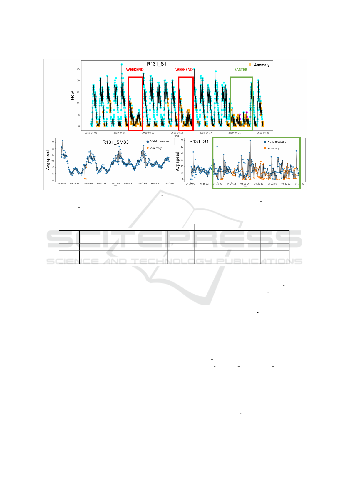
Figure 5: At the top, trafﬁc ﬂow trend of sensor R131 S1 in Exp.3 with anomalies in orange and observations in another

cluster in light blue. At the bottom, the trend of average speed during the Easter period for sensor R131 SM83 on the left side

and sensor R131 S1 on the right side.

Table 2: Results.

Number of sensors with % anomalies

anomalies < 1% from 1% to 5% > 5%

avg anomalies

per sensor

simul.

anomalies

exec. time

(minutes)

Exp.2 2688 17 25 4 55 632 76

Exp.3 1620 25 11 2 33 307 180

Exp.4 5051 15 22 9 103 1418 173

and the observations during the night period are often

classiﬁed as anomalies. We can observe that high val-

ues that are not in line with the normal trend for the

ﬂow or the average speed are labeled as anomalies.

Comparing the two time series, it can be observed

that when the observation is different from the trend

for even just one of the variables (ﬂow or speed), it is

labeled as an outlier.

5.2 Experiment 2

The second experiment takes as input the multivari-

ate time series of measurements produced by all sen-

sors in the selected area. The ST-BDBCAN algorithm

identiﬁes 207 clusters. Table 2 shows the total num-

ber of detected anomalies, the number of sensors with

a very low (lower than 1%), normal (from 1% to 5%)

and high (higher than 5%) percentage of anomalies in

one month, the mean number of anomalies for each

sensor, the number of simultaneous anomalies, and

the execution time in minutes required to evaluate the

anomalies for the whole April month. Simultaneous

anomalies are observations labeled as anomalies that

refer to the same timestamp and belong to different

sensors. The sensors without anomalies are 3. Exp.2

detects only 4 anomalies for sensor R002 S 2 in the

whole month. Besides, sensor R002 S 5, which is lo-

cated in the same crossroad of sensor R002 S2, has a

13% of outliers (375 anomalies). In general, the value

of ﬂow detected by sensor R002 S5 is more than dou-

ble of the ﬂow detected by the other sensors in the

crossroad. This leads to the classiﬁcation of its val-

ues as anomalous even if they are aligned with the

normal trend of the sensor itself. In particular, the

majority of anomalies are detected during the week-

end and the holidays. In Figure 2, the time series of

sensor R002 S5 is compared with the time series of

sensors R002 S1, R002 S2, and R002 S4. It can be

observed that during holidays and weekends the traf-

ﬁc ﬂow measured by R002 S5 is high, while the traf-

ﬁc ﬂow of the other sensors in the crossroad is sig-

niﬁcantly reduced. The high ﬂow values are labeled

as anomalous since they are out of context compared

with the spatial neighbors.

In Exp.1, sensor R002

S2 had a high number of

anomalies because we do not compare its values with

WEBIST 2021 - 17th International Conference on Web Information Systems and Technologies

514

the neighboring sensors but only with its own trend.

When integrating the space dimension and compar-

ing its measurements with the simultaneous measure-

ments of the sensors in the same crossroad, the ma-

jority of observations that are classiﬁed as anomalous

in Exp.1 are contextualized with the neighboring sen-

sors observations and no more classiﬁed as anoma-

lies. However, sensor R002 S5 has a trend that signif-

icantly differs from the other sensors in the crossroad

and its number of anomalies is higher. Generally, it

can be observed that anomalies with very high ﬂow

or speed values are sensor faults and anomalies corre-

sponding to normal values of ﬂow or speed are con-

textual anomalies, as in the case of sensor R002 S5.

5.3 Experiment 3

The third experiment is a modiﬁed version of Exp.2

that was performed to reduce the number of detected

anomalies. In order to do that the values of k and

ST -BDBCAN

MinPts

are increased. As shown in Ta-

ble 2, the number of anomalies is reduced to 1620,

the number of sensors without anomalies is triplicated

and the number of sensors with more than 5% of ob-

servations labeled as outliers is halved compared with

Exp.2. The number of clusters detected by Exp.3

is 25; increasing 5 times the ST -BDBCAN

MinPts

pro-

duced a reduction of around 8 times in the number of

clusters. For sensor R002 S2 zero anomalies are de-

tected and for sensor R002 S5 only one anomaly is

detected. The anomaly is shown in Figure 3 and is a

real anomaly that corresponds to a very high and not

realistic value of average speed.

Therefore, it seems that this solution detects sen-

sor faults or contextual point anomalies instead of

unusual trafﬁc conditions or contextual collective

anomalies. Observing the anomalies detected for sen-

sor R131 S1 (one of the two sensors with a very high

percentage of outliers) in Figure 5, the observations of

weekends and Easter holidays that are unusual traf-

ﬁc conditions are labeled as anomalies. The graph

on the right-bottom shows the trend of Easter holi-

day average speed for sensor R131 S1 highlighting

that the values labeled as anomalous have very strange

values of average speed and can be considered sen-

sor faults. To underline the difference between these

values and the normal values of average speed, on

the left-bottom graph the average speed trend for the

same days of sensor R131 SM83 is displayed. More-

over, we can observe that all the observations of the

sensor R131 S1 from the 1st of April to the 25th of

April belongs to the same cluster since they have

the same color in the top graph of Figure 5. There-

fore, the parameters’ conﬁguration of Exp.3 tends to

identify sensor faults or contextual point anomalies

rather than contextual collective anomalies because

the whole time series is located in the same cluster

and the overall trend can be investigated.

5.4 Experiment 4

The fourth experiment is a modiﬁed version of Exp.2

with a higher value of the p parameter. The percent-

age of anomalies that should be detected (AP) is set

to 3%. As a consequence, the value of ST-BOFUB

decreases from 2 in Exp.2 to 1.68, a lower upper

bound generates more anomalies. Lowering the ST-

BOFUB observations with a lower ST-BOF will be

labeled as anomalies; thus, the number of contextual

collective anomalies will increase and more unusual

trafﬁc conditions will be identiﬁed (e.g. incidents or

trafﬁc jams). Table 2 displays that this conﬁguration

identiﬁes 5051 anomalies and the number of sensors

with a very high percentage of anomalies is doubled

compared with Exp.2; however, the number of sen-

sors with less than 1% of anomalies is only slightly

reduced. The number of clusters (218) slightly in-

creased compared with Exp.2. For sensor R002 S2,

only 5 anomalies are detected, however for sensor

R002 S5 more than 1000 anomalies are identiﬁed.

This conﬁguration of parameters generates different

results for different sensors. In Figure 4, the traf-

ﬁc ﬂow time series of sensor R002 S5 and R031 S2

are displayed with their outliers highlighted in orange.

For sensor R002 S 5, anomalies can be used to identify

weekends, holidays and the night period where traf-

ﬁc ﬂow drops signiﬁcantly. For sensor R031 S2, the

conﬁgured parameters allow detecting all the point

anomalies in the time series but do not highlight un-

usual trafﬁc conditions.

5.5 Discussion

The experiments are performed on data collected by

road trafﬁc sensors; this kind of sensor is particularly

challenging because the trafﬁc ﬂow and the average

speed of vehicles are not continuous phenomena in

the space-time domain. The time series of each sensor

can have a very different amplitude and trend com-

pared with the others in the same area. Moreover, in

the city of Modena, trafﬁc sensors are located near

trafﬁc lights; thus, even if data are aggregated ev-

ery 15 minutes to reduce the effect of the trafﬁc light

logic, the ﬂow and the average speed are strongly in-

ﬂuenced by the viability of the crossroad. Thus, even

if the spatio-temporal distance between two observa-

tions is small the value of the behavioral variables

can be very different. For example, sensor R002 S2

Anomaly Detection in Multivariate Spatial Time Series: A Ready-to-Use Implementation

515

had very few anomalies in all experiments excluding

Exp.1, the reason is that its values of ﬂow are very

low, generally behind 20 vehicles every 15 minutes;

thus, compared with the other sensors that have higher

variability in trafﬁc ﬂow the difference between its

observations is reduced. Although, when the obser-

vations of sensor R002 S2 are considered singularly,

as in Exp.1, the algorithm can recognize anomalous

peaks. Exp.2 demonstrates good performances in de-

tecting sensor faults or point anomalies in the major-

ity of sensors, but when the percentage of anomalies is

very high (above 5%) the detected anomalies also in-

clude unusual trafﬁc conditions. Thus, when the per-

centage of anomalies for a sensor is low (less than

1%) a good solution to ﬁnd unusual trafﬁc conditions

is to perform anomaly detection for that single sensor,

as in Exp.1. The set of parameters of Exp.3 guaran-

tee the identiﬁcation mainly of sensor faults. Indeed,

in Exp.4, both sensor faults and unusual trafﬁc condi-

tions are identiﬁed.

6 CONCLUSIONS

This work describes the implementation of an al-

gorithm able to cluster spatio-temporal data and

recognize different types of anomalies: contextual

point anomalies and contextual collective anoma-

lies. The adopted algorithm combines ST-BOF and

ST-BDBCAN in cascade and has several parameters

which have to be heuristically optimized. Several

tests are needed to deﬁne the set of parameters suit-

able for the application and the type of anomalies

that need to be detected (e.g. sensor faults or sen-

sor unusual behavior). We released a Python imple-

mentation of the algorithm and tested it with differ-

ent conﬁgurations to ﬁnd anomalies on trafﬁc sensor

data in the city of Modena, Italy. The obtained re-

sults are promising and show the potential of consid-

ering the geographical features of the data in anomaly

detection. Thanks to this work, some unresolved

challenges can be highlighted: managing the spatio-

temporal distance is quite complicated and could ben-

eﬁt from more sophisticated distance functions able

to capture the topology of the street, the trafﬁc corre-

lations, and assign optimized weights to the features.

Still, this work could be a baseline for future improve-

ments. In order to reduce the execution time of the

algorithm, in the future, we will work on the imple-

mentation of Approx-ST-BDBCAN, which is the par-

allelized version of the algorithm described in (Dug-

gimpudi et al., 2019).

REFERENCES

Bachechi, C. and Po, L. (2019). Implementing an urban

dynamic trafﬁc model. In 2019 IEEE/WIC/ACM In-

ternational Conference on Web Intelligence, WI 2019,

Thessaloniki, Greece, October 14-17, 2019, pages

312–316. ACM.

Bachechi, C., Rollo, F., and Po, L. (2020). Real-time data

cleaning in trafﬁc sensor networks. In 17th IEEE/ACS

International Conference on Computer Systems and

Applications, AICCSA 2020, Antalya, Turkey, Novem-

ber 2-5, 2020, pages 1–8. IEEE.

Bachechi, C., Rollo, F., and Po, L. (2021). Detection and

classiﬁcation of sensor anomalies for simulating urban

trafﬁc scenarios. Clust. Comput. to appear.

Breunig, M. M., Kriegel, H., Ng, R. T., and Sander, J.

(2000). LOF: identifying density-based local outliers.

In Chen, W., Naughton, J. F., and Bernstein, P. A., edi-

tors, Proceedings of the 2000 ACM SIGMOD Interna-

tional Conference on Management of Data, May 16-

18, 2000, Dallas, Texas, USA, pages 93–104. ACM.

Celik, M., Dadaser-Celik, F., and Dokuz, A. (2011).

Anomaly detection in temperature data using dbscan

algorithm.

Desimoni, F., Ilarri, S., Po, L., Rollo, F., and Trillo-Lado,

R. (2020). Semantic trafﬁc sensor data: The trafair

experience. Applied Sciences, 10(17).

Duan, L., Xu, L., Guo, F., Lee, J., and Yan, B. (2007). A

local-density based spatial clustering algorithm with

noise. Inf. Syst., 32(7):978–986.

Duggimpudi, M. B., Abbady, S., Chen, J., and Raghavan,

V. (2019). Spatio-temporal outlier detection algo-

rithms based on computing behavioral outlierness fac-

tor. Data & Knowledge Engineering, 122:1–24.

Ester, M., Kriegel, H.-P., Sander, J., and Xu, X. (1996).

A density-based algorithm for discovering clusters in

large spatial databases with noise. In Proceedings of

the Second International Conference on Knowledge

Discovery and Data Mining, KDD’96, page 226–231.

AAAI Press.

Gupta, M., Gao, J., Aggarwal, C. C., and Han, J. (2014).

Outlier detection for temporal data: A survey. IEEE

Trans. Knowl. Data Eng., 26(9):2250–2267.

Po, L., Rollo, F., Bachechi, C., and Corni, A. (2019a). From

sensors data to urban trafﬁc ﬂow analysis. In 2019

IEEE International Smart Cities Conference, ISC2

2019, Casablanca, Morocco, October 14-17, 2019,

pages 478–485. IEEE.

Po, L., Rollo, F., Viqueira, J. R. R., Lado, R. T., Bigi,

A., L

opez, J. C., Paolucci, M., and Nesi, P. (2019b).

TRAFAIR: understanding trafﬁc ﬂow to improve air

quality. In 2019 IEEE International Smart Cities Con-

ference, ISC2 2019, Casablanca, Morocco, October

14-17, 2019, pages 36–43. IEEE.

Rollo, F., Sudharsan, B., Po, L., and Breslin, J. (2021). Air

quality sensor network data acquisition, cleaning, vi-

sualization, and analytics: A real-world iot use case.

In Proceedings of the 2021 ACM International Joint

Conference on Pervasive and Ubiquitous Comput-

ing and Proceedings of the 2021 ACM International

WEBIST 2021 - 17th International Conference on Web Information Systems and Technologies

516

Symposium on Wearable Computers, UbiComp/ISWC

2021 Adjunct, Virtual, USA, September 21-26, 2021.

ACM. to appear.

Wang, H., Bah, M. J., and Hammad, M. (2019a). Progress

in outlier detection techniques: A survey. IEEE Ac-

cess, 7:107964–108000.

Wang, Z., Song, G., and Gao, C. (2019b). An isolation-

based distributed outlier detection framework using

nearest neighbor ensembles for wireless sensor net-

works. IEEE Access, 7:96319–96333.

Anomaly Detection in Multivariate Spatial Time Series: A Ready-to-Use Implementation

517