Path Following with Deep Reinforcement Learning for Autonomous Cars

Khaled Alomari

, Ricardo Carrillo Mendoza, Daniel Goehring and Ra

ul Rojas

Dahlem Center for Machine Learning and Robotics - Freie Universit

at Berlin, Arnimallee 7, 14195 Berlin, Germany

Keywords:

Deep Reinforcement Learning, Deep Deterministic Policy Gradient, Path-following, Advanced Driver

Assistance Systems, Autonomous Vehicles.

Abstract:

Path-following for autonomous vehicles is a challenging task. Choosing the appropriate controller to apply

typical linear/nonlinear control theory methods demands intensive investigation on the dynamics and kinemat-

ics of the system. Furthermore, the non-linearity of the system’s dynamics, the complication of its analytical

description, disturbances, and the inﬂuence of sensor noise, raise the need for adaptive control methods for

reaching optimal performance. In the context of this paper, a Deep Reinforcement Learning (DRL) approach

with Deep Deterministic Policy Gradient (DDPG) is employed for path tracking of an autonomous model

vehicle. The RL agent is trained in a 3D simulation environment. It interacts with the unknown environment

and accumulates experiences to update the Deep Neural Network. The algorithm learns a policy (sequence

of control actions) that solves the designed optimization objective. The agent is trained to calculate heading

angles to follow a path with minimal cross-track error. In the ﬁnal evaluation, to prove the trained policy’s

dynamic, we analyzed the learned steering policy strength to respond to more extensive and smaller steering

values with keeping the cross-track error as small as possible. In conclusion, the agent could drive around

the track for several loops without exceeding the maximum tolerated deviation, moreover, with reasonable

orientation error.

1 INTRODUCTION

Autonomous driving has gained exceptional atten-

tion as an essential research topic in recent years.

It is forming the future of transportation. This ten-

dency is the product of the increased efforts from sev-

eral automotive manufacturers to integrate more Ad-

vanced Driver Assistance Systems (ADAS) with var-

ious automation features in their modern cars. More-

over, they endeavor to test them on public roads

around the globe to test their stability under envi-

ronmental uncertainties (Chan, 2017). To develop

fully autonomous cars, High-performance assistance

systems are needed; developing them demands in-

tensive investigation on the dynamics and kinemat-

ics states of the system under a wide range of driving

conditions in complex environments (Martinsen and

Lekkas, 2018).

Choosing the appropriate controller, applying typ-

ical linear/nonlinear control theory methods, is not

always possible due to the non-linearity of the dy-

namics, sensor noise inﬂuence, disturbances, and

unknown parameters. Thus, artiﬁcial intelligence ap-

https://orcid.org/0000-0001-7248-0056

proaches to design an adaptive controller that can

reach optimal performance were raised. Reinforce-

ment learning is a framework by which a control pol-

icy can be found for a system with unknown dynam-

ics (Hall et al., 2011) (Calzolari et al., 2017).

2 RELATED WORK

Reinforcement Learning (RL) is a category of ma-

chine learning in which an agent learns from interact-

ing with an environment (i.e., the agent accumulates

the perception about the environment from experi-

mental trials and simple relative feedback received).

The goal is to let the agent learn the best possible ac-

tions in an environment to attain its goals efﬁciently.

During the process, the agent is capable of adapting to

the environment to maximize future rewards actively

(Sutton and Barto, 2018)(Kaelbling et al., 1996).

In (Wang et al., 2018), TORCS environment was

used to train an RL-agent. Their goal was to drive

the car at high speed in the center of the road without

crashing other cars. A set of sensor data, including

track points, car speed, orientation, and the deviation

between the vehicle’s longitudinal axis and the ideal

Alomari, K., Mendoza, R., Goehring, D. and Rojas, R.

Path Following with Deep Reinforcement Learning for Autonomous Cars.

DOI: 10.5220/0010715400003061

In Proceedings of the 2nd International Conference on Robotics, Computer Vision and Intelligent Systems (ROBOVIS 2021), pages 173-181

ISBN: 978-989-758-537-1

173

track, are used as inputs for an adopted DDPG algo-

rithm. Decisions are made for either no throttle or full

throttle, no braking or full braking, or full steering to

the left or the right.

In contrast to the previous approach, Jaritz et al.

(Jaritz et al., 2018) proposed to learn the end-to-end

driving control of an autonomous car using only im-

ages from a forward-facing monocular camera. They

trained the agent in a simulated environment to learn

full control -steering, brake, gas, and even hand brake

to a pressure drifting- using the A3C algorithm. Sim-

ilarly, in (Kendall et al., 2018), they used the monoc-

ular images to train an agent to follow a lane. In (Li

et al., 2019), a perception module in the form of a

Convolutional Neural Network (CNN) is utilized to

extract track information from the image data of a rac-

ing simulator. This information is then combined with

information about the driving condition, such as ve-

hicle position, speed, and orientation, to train an RL

agent using DPG to predict a continuous steering an-

gle.

Reinforcement Learning methods are incredibly

time-consuming, and millions of experiences need to

be accumulated to learn complicated tasks accurately.

As a consequence, most of the successfully robotic

RL agents are trained in a simulation environment.

As a result, the training process can be automated ef-

ﬁciently, and the dangerous circumstances caused by

trial-and-error are reserved from the real world. Still,

The RL agent should be tested in a real situation.

In this paper, the state-of-the-art DRL algorithm

Deep Deterministic Policy Gradient is employed for

path tracking control of an autonomous model ve-

hicle. The RL agent is trained in a 3D simulation

environment. It interacts with the anonymous envi-

ronment and accumulates experiences to update the

Deep Neural Network. The agent is trained to gener-

ate and execute heading angles to follow a path with

a minimum cross-track error. The deviation between

the target and actual path is mainly considered, which

could be signiﬁcantly reduced. The beneﬁt of our im-

plementation is that it brings close the implementa-

tion from simulation to real-world application. More-

over, the simulator engine used has dynamic parame-

ters which make the training closer to reality. It also

has other sensors used in autonomous driving, such as

LIDAR, stereo camera, and odometry.

3 METHODS AND SETUP

This section describes in detail the methods used to

implement the environment and the reinforcement

learning agent.

3.1 Environment Setup

This subsection describes the setting up of an envi-

ronment to apply and test RL-agent. The built envi-

ronment integrates the AutoMiny-simulator (Schmidt

et al., 2019) with the open-source library OpenAI

Gym (Brockman et al., 2016). In the following,

the environment structure will be described in detail,

along with the AutoMiny-simulator.

3.1.1 AutoMiny Simulator

The AutoMiny-Simulator is integrated with ROS and

is based on the robust physics engine Gazebo. It cre-

ates a comprehensive 3D dynamic robot environment

capable of recreating the physical driving setup of the

agent. Furthermore, it emulates dynamic parameters

such as static and dynamic friction and aerodynam-

ics. It considers the vehicle dynamics parameters like

wheel acceleration, wheel material, and torque, mak-

ing it more reliable to transfer the developed algo-

rithms into the model car and test them.

The simulator is developed based on the ex-

isting AutoMiny project at the Freie University of

Berlin (Alomari et al., 2020). It provides all nodes and

topics used by the physical AutoMiny car (Schmidt

et al., 2019). The Kinematic model of the car has

been parameterized using its URDF description. All

the onboard sensors associated with AutoMiny, like

the RGBD camera, IMU, and the laser scanner, are

provided in the simulated car.

3.1.2 GazeboAutominyEnv

The developed environment, named ”GazeboAu-

tominyEnv,” links the AutoMiny-simulator with the

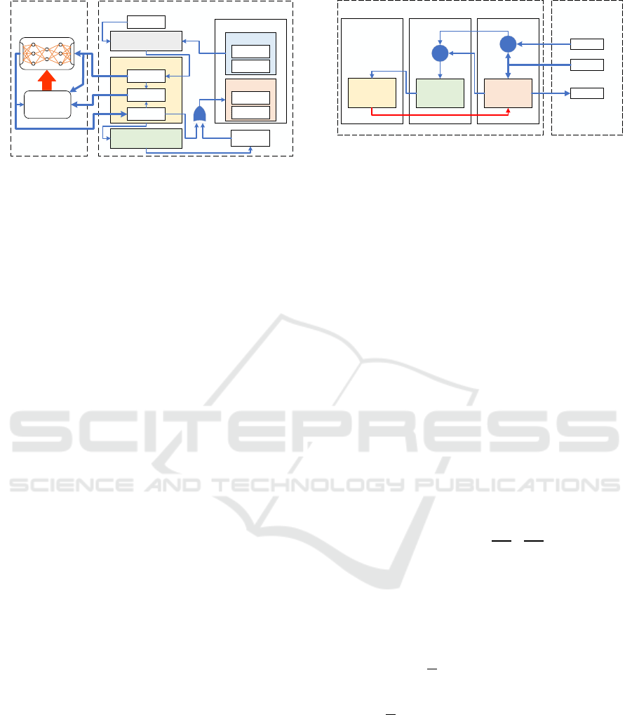
open-source library OpenAI Gym. Figure 1 describes

the structure of the developed environment. First, the

simulator is launched while initializing the environ-

ment class. Then, at the rate of 30 Hz, the observation

function inquires raw observation data from the sim-

ulator by subscribing to pre-deﬁned suitable topics.

Moreover, it calls the path points. Finally, the obser-

vation function collects data and returns them normal-

ized in a box form (continuous values).

At each iteration, the step function requests the

last observation data. This supplied information de-

ﬁnes a target point on the path and formalizes a time-

related state. The state-space is fed to both the actor

and the critic networks. The actor-network processes

this data and predicts an action based on the policy.

The estimated action is sent back to the environment

and supplied to the critic network as well. The step

function controls the action and publishes it to the

ROBOVIS 2021 - 2nd International Conference on Robotics, Computer Vision and Intelligent Systems

174

RL‐Agent

State

Reward

Reset

Action

Step

Position

correction

Environment

Policy

Reinforcement

learning

algorithm

Policy

update

Simulator

Subscriber

Localization

IMU

Publisher

Steering

Speed

XOR

Observation

Trajectory

(DDPG)

Figure 1: GazeboAutominyEnv Environment Setup Struc-

ture; At each iteration, the step function fed the state param-

eters to the RL-agent, which predicts an action based on the

policy. The estimated action is sent back to the step func-

tion to process it. After taking action, the reward function

evaluates the new error value and either reward the action

or penalize it.

simulator topics. After taking action, the step func-

tion requests new observation data. This data is used

to update the state and calculate the error between the

estimated and actual controlled value. Meantime, it

evaluates this error value and either reward the action

or penalize it. The reward value is delivered to the

critic network. The critic network then updates the

policy. However, the process on the agent side will be

described more in detail in Section 3.2.

Once the episode is completed or terminated, the

step function calls the reset function, which moves the

agent back to an initial position (either ﬁxed or ar-

bitrary) using a navigation system based on a vector

virtual force ﬁeld (Alomari et al., ress).

3.2 Design of the RL-agent

For this work, the Deep Deterministic Policy Gra-

dient (Lillicrap et al., 2016) is employed. It is one

of the straightforward algorithms in Deep Reinforce-

ment Learning, which is suitable for continuous and

discrete action spaces. Furthermore, DDPG has an

actor-critic architecture and concurrently learns a pol-

icy and a Q-function. The agent implementation is

utilized by Keras-rl. Keras-rl operates with the Ope-

nAI Gym environment. The deep learning part is ac-

complished in the Keras framework with TensorFlow

backend and allows us to establish custom actor-critic

networks.

Figure 2 presents the basic structure of the imple-

mentation of the reinforcement learning agent. The

process in the agent can be classiﬁed into three ma-

jor simultaneous processes. In rule one, the actor-

network µ(s|θ

) in the RL agent receives a state s

from the environment, predicts an action a

based on

this state and using the policy learned, and passes it

MemoryMemory

Replay

Buffer

Memory

Replay

Buffer

EnvironmentEnvironment

StateState

RewardReward

ActionAction

PredictionPrediction

Actor-critic

Networks

Learning

Target

Actor-critic

Networks

DDPG

Update Weights

N Sample

Experiences

action

State / reward

Figure 2: DDPG agent Setup Structure.

(with additional noise N ) to the environment for ex-

ecution, as shown in Equation 1.

= µ(s|θ

) + N

(1)

Consequently, both the state received from the

environment and the predicted action are fed to the

critic-network Q(s, a|θ

) to estimate an action-state

value function Q(s, a). Once the agent ends up in

a new state s

t+1

, an experience tuple consisting of

state, action, reward, and follower state (s

, a

, r

, s

t+1

)

is collected in a ﬁnite-sized cache known as replay

buffer. When the replay buffer is full, it discards the

oldest samples and stores new ones. In rule three, a

minibatch sample of size N from the collected experi-

ence in the replay buffer is delivered to a copy of the

actor-critic networks. The copy architecture is known

as target-actor µ

(s|θ

) and target-critic Q

(s, a|θ

)

networks. Those networks are used to predict for each

sample i ∈ N of the minibatch an output y

based on

the Equation 2 (Lillicrap et al., 2016):

= r

+ γQ

i+1

, µ

i+1

|θ

)

{z }

i+1

|θ

) (2)

Then, the predicted values are used to calculate

the loss function in Equation 3 (Lillicrap et al., 2016)

and update the critic network weights by minimizing

the loss. While the actor policy is updated using the

sampled policy gradient shown in Equation 4:

L =

∑

−Q(s

, a

|θ

))

(3)

∇

θµ

J ≈

∇

Q(s, a|θ

s=s

,a=µ(s

)

∇

θµ

µ(s|θ

(4)

A feedforward, fully-connected Multi-Layer-

Perceptron ANN structure with two hidden layers is

used for both actor and critic networks. Rectiﬁed Lin-

ear Unit (ReLU) activation function is applied to all

neurons in the hidden layers. The output layer is then

either the action the agent can perform or the state-

action value function. Tangent-hyperbolic (tanh) ac-

tivation function is employed to neurons in the output

layers of both structures.

Path Following with Deep Reinforcement Learning for Autonomous Cars

175

map

Lookahead distance

Target

point

Closest

point

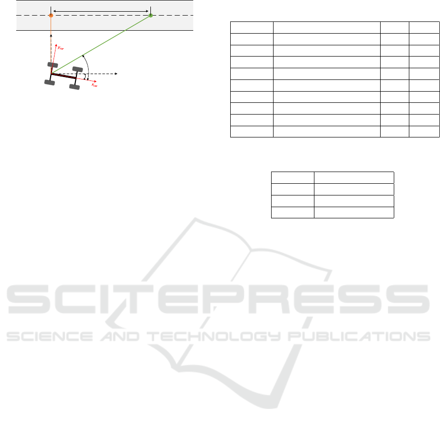
Figure 3: Path following task setup; the agent is trained to

follow a given path by controlling its steering. Besides the

distance to the target e

, the cross-track-error e

is measured

and minimized.

The actor-network is used to learn the determinis-

tic policy of the DDPG agent, where an explicit ac-

tion a is determined directly based on the car obser-

vation data and the target point. The critic network

learns state-action value function Q based on the cur-

rent state and the action selected in it. The action was

not included until the second hidden layer of the critic

network. Both the number of neurons in the hidden

layers of the ANN, besides the learning rate, are ar-

bitrarily selectable hyperparameters. The Ornstein-

Uhlenbeck (OU) noise process, added to the action

to guarantee the agent’s exploration, is deﬁned by the

parameters θ = 0.15, µ = 0, and σ = 0.2.

3.3 Path Following Setup

Besides the distance to the target, the agent learns

to minimize the cross-track error to achieve the best

match between the driving path and the desired one.

Figure 3 simulates the agent in one of the possible

states. The agent is supposed to drive at a constant

speed and interact with an anonymous environment

to explore it, attempting to reach a target point. While

the agent is moving, the desired target will be updated

continuously with all other parameters, and based on

the reward function, it receives either a reward or a

penalty. In addition, the agent is modifying its orien-

tation by controlling its steering based on the reward

it receives.

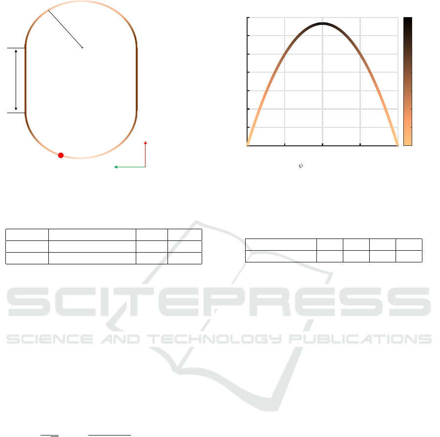
Figure 4a shows the middle points of the path that

will be used to train the agent. Using several points

to train the agent will enhance its performance when

tested on other trajectories. The agent will learn how

to approach points by steering left and points on his

longitudinal axis. Still, due to the limitation of the

map, the agent might fail on the tracks that have the

right turns. The desired speed is estimated based on

the orientation error between the agent and the target

point. Figure 4b shows the relationship between the

target speed and the orientation error.

Table 1: Observation data provided through the environ-

ment.

Symbol Description Min Max

x [m] Car position on x axis -0.1 6.30

y [m] Car position on y axis -0.1 4.50

ψ [rad] Car orientation yaw −π +π

[m/s] Car speed on x axis -0.0 +0.8

[m/s] Car speed on y axis -0.0 +0.1

[m] Target position on x axis -0.1 6.30

[m] Target position on y axis 0.1 4.50

[rad] Target orientation yaw −π +π

[m/s] Target linear speed 0.0 +0.8

Table 2: List of error measured by the environment step

function.

Symbol Description

Distance to target

Cross track error

Orientation error

The RL agent demands to get all associated infor-

mation about the current state of the environment to

calculate the control components and accomplish the

mission. The environment provides various contin-

uous vehicle state variables and sensors data. How-

ever, the main goal is to train the agent with as few as

possible low-dimensional data. The symbols of state

variables distinguished as necessary, including a short

description and the value range used for data prepro-

cessing, are shown in Table 1. (x, y) describes the cur-

rent position of the vehicle at the midpoint of the rear

axle, where (v

, v

) are the linear vehicle speed vec-

tor components. ψ

deﬁnes the rotational movement

of the vehicle around the vertical axis of the vehicle

coordinate system. (x

, y

, ψ

) are the target point and

orientation respectively. v

is the target speed.

Furthermore, various error measures are available,

which will be used to design the RL agents’ reward

function. Table 2 shows a list of error quantities cal-

culated in the state. e

is longitude to the Target po-

sition. In contrast, the cross-track error e

describes

the deviation from the nominal to the actual path, and

the yaw angle error e

describes the deviation in the

alignment of the vehicle. All observation quantities

and errors are normalized.

One of the key advantages of using DDPG is its

ability to operate over continuous action spaces. In

the studied challenge, the agent learns a continuous

steering angle, which can assume any value between

[−0.78, +0.95] rad. Table 3 shows the value range for

action space

Rewards are calculated each time step t after tak-

ing action a. It can be viewed as a feedback ﬂag that

evaluates how good taking action a in state s is. In this

ROBOVIS 2021 - 2nd International Conference on Robotics, Computer Vision and Intelligent Systems

176

map

L = 2 m

R = 1.65 m

(a)

-1 -0.5 0 0.5 1

[normalized]

0.05

0.1

0.15

0.2

0.25

0.3

0.35

Desired speed

0.05

0.1

0.15

0.2

0.25

0.3

0.35

(b)

Figure 4: (a) The path used to train the RL-agents, (b) beside the function used to predict the desired speed, while the actual

speed value before normalization can be found in Table 1.

Table 3: RL-agents continuous action space.

Symbol Description Min Max

δ [rad] Steering Command -0,78 +0,95

v [m/s] Speed Command -0.0 +0,8

task, two main errors should be minimized in each

step: the vehicle’s orientation error and the deviation

between the target and actual path of the vehicle, since

the vehicle should deviate as little as possible from

the planned line of the path planner. Therefore, the

reward function should evaluate both e

and e

r(t) = r(e

) + r(e

) (5)

However, the cross-track error needs to be limited

to end the training episode and reset the agent once

exceeding it.

r =

(

−10 if e

> D

√

2π

exp(−

((e

)−µ)

2σ

) else

(6)

A Gaussian distribution is used to determine the

rewards component, shifted by -1 with mean value

µ = 0 and standard deviation σ = 0.2.

The network structure mentioned in 3.3, and Ta-

ble 4 presents the number of neurons used in the hid-

den layers for both networks. The learning process

applied is Adam with a learning rate of 10

−4

and

−3

for the actor and critic networks, respectively.

A discount factor of γ = 0.99, and for soft target up-

dates τ = 10

−3

were used. The random noise process

was added to the action output value to guarantee the

agent’s exploration during the whole training proce-

dure. It is deﬁned by the parameters θ = 0.15, µ = 0,

and σ = 0.2.

Table 4: Number of neurons used in hidden layers for the

actor and critic networks.

Architecture 1 400 300 400 300

4 EVALUATION

The training is set to 120 000 steps and elaborated as

a continuous task. i.e., no maximum number of steps

per episode is deﬁned. The episode ends only when

the cross-track-error is higher than a speciﬁc value (D

= 20 cm). When the agent exceeds the deﬁned cross-

track error, the learning process pauses, and the agent

position is set back close to the track again. Only then

does the training resume. The maximum allowed de-

viation of the target path is chosen based on the map

size and the function’s capabilities that reset the agent

position.

4.1 Reward Function Evaluation

Considering Figure 3, the setup includes three main

errors. The euclidean distance to the target point e

the cross-track error e

, and the orientation error e

In this experiment, we will study the effect of com-

bining e

with e

in the reward function R(e

, e

), and

compare the result with using reward function R(e

)

that only consider the e

Table 5 presents a quick review of the setup used

to train the agents. For both agents, a ﬁxed lookahead

offset of 60 cm is deﬁned, the same network structure,

shown in Table 4 is used. Furthermore, both used the

observation space shown in Table 1. The agents were

tasked to obtain proper steering policies.

Path Following with Deep Reinforcement Learning for Autonomous Cars

177

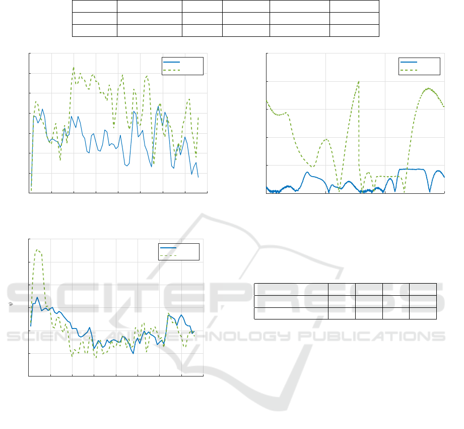
Table 5: Comparison, of setup used to train RL-agents to verify the reward function.

Observation Action Reward Lookahead Network

Agent 1 Table 1 δ R(e

, e

) 60 [cm] Table 4

Agent 2 Table 1 δ R(e

) 60 [cm] Table 4

0 10 20 30 40 50 60 70 80

Loop

0.03

0.04

0.05

0.06

0.07

0.08

0.09

0.1

Mean e

[m]

agent 1

agent 2

(a)

0 10 20 30 40 50 60 70 80

Loop

-0.1

0.1

0.2

0.3

0.4

0.5

Mean e [rad]

agent 1

agent 2

(b)

Figure 5: Comparison of the two RL-agents performance

during training for 76 loops with lookahead offset of 60 cm;

(a) the mean cross-track error over each loop of the training.

(b) the mean orientation error vs. training loops.

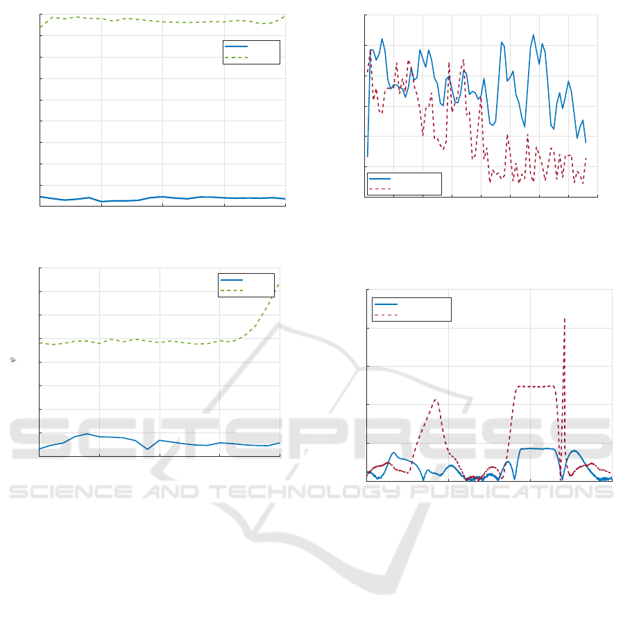
Both agents were trained for 76 loops around the

path. In Figure 5, the mean orientation error e

, and

mean cross-track error e

are plotted vs. loops over

the whole training for both agents. As we can spot out

from the ﬁgure, integrating the cross-track error in the

reward function enhanced the agent’s ability to drive

closer to the target path without affecting the orien-

tation error. Nevertheless, both agents could drive

around the path for a full loop by the end of the train-

ing.

In order to evaluate the performance of both

agents, they were both tested after the end of the train-

ing. The idea was to let them drive around the path

0 500 1000 1500

Step

0.05

0.1

0.15

0.2

0.25

[m]

agent 1

agent 2

Figure 6: Comparison of the two RL-agents performance

during testing for one loop with lookahead offset of 60 cm;

the cross-track error over one loop of the testing.

Table 6: Number of hidden layers neurons in each RL-

agent.

Architecture 1 400 300 400 300

Architecture 2 600 450 600 450

for several loops and measure the Root-Mean-Square

(RMS) for the orientation error and the cross-track er-

ror and compare the results of a quantitative perspec-

tive. Then, in the main time, observe the changes of

both errors during one loop drive.

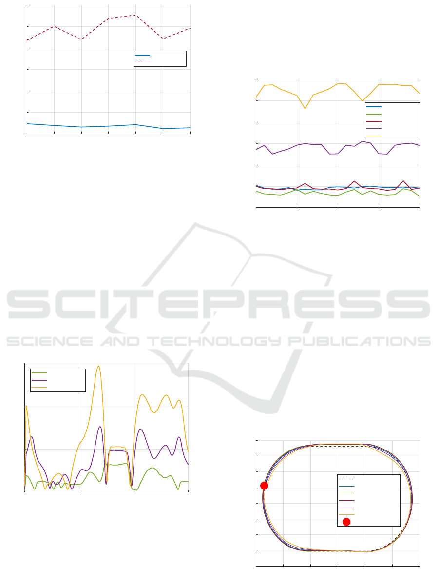
Figure 6 plots the variations of the cross-track er-

ror during the second loop of the test. In the ﬁgure,

it is shown that agent 1 showed more steady perfor-

mance in keeping the car close to the path than agent

2. Moreover, agent 2 failed to ﬁnish one loop around

the track, and a reset position was needed to put it

back close to the track. Figure 7 shows the RMS error

over the 20 loops of the testing for both agents. As a

result, we can assess the performance of both agents

over the whole testing period.

4.2 Neural Network Evaluation

In this experiments, different agents with various neu-

ral network architectures were trained to learn the

steering policy. Two of them outperformed the other

ones. In the following, the victorious agent’s results

will be compared. Table 6 shows the number of hid-

den layers neurons in each RL-agent.

ROBOVIS 2021 - 2nd International Conference on Robotics, Computer Vision and Intelligent Systems

178

0 5 10 15 20

Loop

0.03

0.04

0.05

0.06

0.07

0.08

0.09

0.1

0.11

RMS(e

) [m]

agent 1

agent 2

(a)

0 5 10 15 20

Loop

0.14

0.15

0.16

0.17

0.18

0.19

0.2

0.21

0.22

RMS(e ) [rad]

agent 1

agent 2

(b)

Figure 7: Comparison of the two RL-agents performance

during testing for 20 loops with lookahead offset of 60 cm;

(a) the RMS cross-track error over 20 loops during testing.

(b) the RMS orientation error vs. 20 loops.

Both agents learned on the same reward function

R(e

, e

), and were trained for 76 loops with a ﬁxed

lookahead offset of 60 cm. Furthermore, both used

the observation space shown in Table 1. Finally, the

agents were tasked to obtain proper steering policies.

In Figure 8, the mean cross-track error e

is plotted vs.

loops over the whole training for both agents. As we

can spot out from the ﬁgure, the agent used architec-

ture 2 could remain a small cross-track error by the

end of the training. Nevertheless, both agents could

drive around the path for a full loop by the end of the

training.

In order to evaluate the performance of both

agents, they were both tested after the end of the train-

ing. The idea was to let them drive around the path for

several loops and measure, at each loop, the RMS for

the orientation error, as well as the cross-track error

and compare the results of a quantitative perspective.

0 10 20 30 40 50 60 70 80

Loop

0.02

0.03

0.04

0.05

0.06

0.07

0.08

Mean e

[m]

architecture 1

architecture 2

Figure 8: Comparison of the two RL-agents performance

during training for 76 loops with lookahead offset of 60 cm;

the mean cross-track error over each loop of the training.

0 500 1000 1500

Step Number

0.05

0.1

0.15

0.2

0.25

[m]

architecture 1

architecture 2

Figure 9: Comparison of the two RL-agents performance

during testing for one loop with lookahead offset of 60 cm;

the cross-track error over one loop of the testing.

In the main time, observe the changes of both errors

during one loop drive.

Figure 9 plot the variations of the cross-track error

during the second loop of the test. As can be noticed

from the Figure, the agent with architecture 1 showed

more steady performance in keeping the car close to

the path than agent 2. Moreover, the agent with ar-

chitecture 2 failed to ﬁnish one loop around the track.

A reset position was needed to put it back close to

the track at the ﬁnal curvature of the path. Figure 10

shows the RMS(e

) over the 6 loops of the testing for

both agents. As a result, we can assess the perfor-

mance of both agents over the whole testing period.

The training of the agent with architecture 2 was

repeated with a double number of training steps. Still,

it was not able to show a better performance than the

presented one. For this reason, we will not consider it

in any further evaluation.

Path Following with Deep Reinforcement Learning for Autonomous Cars

179

0 1 2 3 4 5 6

Loop

0.02

0.03

0.04

0.05

0.06

0.07

0.08

RMS(e

)[m]

architecture 1

architecture 2

Figure 10: Comparison of the two RL-agents performance

during testing for 6 loops with lookahead offset of 60 cm;

the RMS cross-track error over 6 loops during testing.

4.3 Further Evaluation

The presented experiments conﬁrmed the importance

of rewarding the cross-track error besides the orienta-

tion error in the path tracking tasks. Agent 1 showed

an exceptional performance during testing the agent.

However, we still need to prove how dynamic the

trained agent is for changes, e.g., the lookahead dis-

tance. For this reason, the agent will be tested for dif-

ferent lookahead distances (20, 40, 80, 100) cm. By

modifying the lookahead distance, we can analyze the

agent’s steering policy strength to respond for more

extensive and smaller steering values with keeping the

cross-track error as small as possible.

0 500 1000 1500

step

0.05

0.1

0.15

[rad]

lookahead 20

lookahead 80

lookahead 100

Figure 11: Testing RL-agents performance For different

lookahead offset values;the cross-track error over one loop

of the testing.

Figure 11 shows the measured errors over one

loop during the proposed test, for some elected looka-

head offset of (20, 80, 100) cm, quantitatively. Thus,

the agent was able to drive around the track with-

out exceeding the maximum tolerated deviation (D =

20cm). Moreover, the orientation error variation is

also in an acceptable range. However, to evaluate

the test more reasonably, the test was held for several

loops, and the mean error (e

and e

) over each loop,

for the whole testing period, is measured and plotted

in Figure 12.

0 5 10 15 20

Loop

0.01

0.02

0.03

0.04

0.05

0.06

0.07

Mean e

[m]

lookahead 60

lookahead 20

lookahead 40

lookahead 80

lookahead 100

Figure 12: Comparison of the RL-agents performance dur-

ing testing for 20 loops with different lookahead offset; (a)

the RMS cross-track error over 20 loops during testing.

After quantitatively evaluating the agent, it is time

to evaluate it qualitatively. In Figure 13, The routes

the agent drove during testing for one loop with dif-

ferent lookahead offset are plotted as well as the op-

timal route. As we can see, the routes are very close

to each other. In order to summarize this plot infor-

mation, the mean and the Standard Deviation (SD) for

each route are shown in Table 7.

5 CONCLUSIONS

In the context of this paper, the state-of-the-art deep

reinforcement learning algorithm DDPG was selected

0 1 2 3 4 5 6

map

[m]

0.5

1.5

2.5

3.5

map

[m]

optimal trajectory

trained lookahead

lookahead 20

lookahead 40

lookahead 80

lookahead 100

starting point

Figure 13: Agent’s driven route during testing, with differ-

ent lookahead testing, together with the optimal path.

ROBOVIS 2021 - 2nd International Conference on Robotics, Computer Vision and Intelligent Systems

180

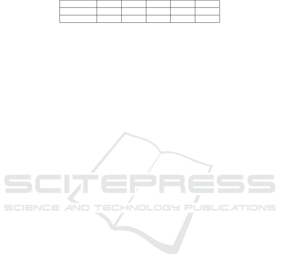
Table 7: Mean and Standard Deviation values for testing the RL-agent with different lookahead offset.

Lookahead 60 20 40 80 100

Mean 0.0195 0.0164 0.0188 0.0391 0.0671

SD 0.0141 0.0090 0.0110 0.0190 0.0398

as an end-to-end learning approach to take over the

comprehensive steering control for an autonomous

vehicle. The proposed agent has been trained and

tested in the AutoMiny-Gazebo environment, which

implements a realistic model of the AutoMiny model

car. The target point was updating continuously in

each iteration during training. The aim was to en-

courage the agent to follow a pre-deﬁned path with a

minimum cross-track error. A continuous state space

includes the agent position, orientation, speed, and

the target point coordinates, and the desired orienta-

tion was employed. Both cross-track error and ori-

entation error were combined in the reward function.

Updating the target points during training made the

agent gain more experience and drove a complete

loop around the track after 80 training loops. Al-

though the achieved results seem very encouraging,

more testing is necessary to validate the agent’s abil-

ity to follow different paths with more diverse route

proﬁles. Moreover, enhance the approach to include

computing the optimal velocity of the vehicle depend-

ing on the path and deploying the agent in a real plat-

form.

ACKNOWLEDGEMENTS

This material is based upon work supported by the

Bundesministerium fur Verkehr und digitale Infras-

truktur (BMVI) in Germany as part of the Shut-

tles&Co project, within the Automatisiertes, Vernet-

ztes Fahren (AVF) program.

REFERENCES

Alomari, K., Carrillo Mendoza, R., Sundermann, S.,

ohring, D., and Rojas, R. (2020). Fuzzy logic-based

adaptive cruise control for autonomous model car. In

ROBOVIS.

Alomari, K., Sundermann, S., G

ohring, D., and Rojas, R.

(in press). Design and experimental analysis of an

adaptive cruise control. Springer CCIS book series.

Brockman, G., Cheung, V., Pettersson, L., Schneider, J.,

Schulman, J., Tang, J., and Zaremba, W. (2016). Ope-

nai gym.

Calzolari, D., Sch

urmann, B., and Althoff, M. (2017).

Comparison of trajectory tracking controllers for au-

tonomous vehicles. In 2017 IEEE 20th Interna-

tional Conference on Intelligent Transportation Sys-

tems (ITSC), pages 1–8.

Chan, C.-Y. (2017). Advancements, prospects, and impacts

of automated driving systems. International Journal

of Transportation Science and Technology, 6(3):208 –

216. Safer Road Infrastructure and Operation Man-

agement.

Hall, J., Rasmussen, C. E., and Maciejowski, J. (2011). Re-

inforcement learning with reference tracking control

in continuous state spaces. In 2011 50th IEEE Confer-

ence on Decision and Control and European Control

Conference, pages 6019–6024.

Jaritz, M., de Charette, R., Toromanoff, M., Perot, E., and

Nashashibi, F. (2018). End-to-end race driving with

deep reinforcement learning. CoRR, abs/1807.02371.

Kaelbling, L. P., Littman, M. L., and Moore, A. P. (1996).

Reinforcement learning: A survey. Journal of Artiﬁ-

cial Intelligence Research, 4:237–285.

Kendall, A., Hawke, J., Janz, D., Mazur, P., Reda, D., Allen,

J., Lam, V., Bewley, A., and Shah, A. (2018). Learn-

ing to drive in a day. CoRR, abs/1807.00412.

Li, D., Zhao, D., Zhang, Q., and Chen, Y. (2019). Re-

inforcement learning and deep learning based lat-

eral control for autonomous driving [application

notes]. IEEE Computational Intelligence Magazine,

14(2):83–98.

Lillicrap, T. P., Hunt, J. J., Pritzel, A., Heess, N., Erez, T.,

Tassa, Y., Silver, D., and Wierstra, D. (2016). Con-

tinuous control with deep reinforcement learning. In

Bengio, Y. and LeCun, Y., editors, 4th International

Conference on Learning Representations, ICLR 2016,

San Juan, Puerto Rico, May 2-4, 2016, Conference

Track Proceedings.

Martinsen, A. B. and Lekkas, A. M. (2018). Curved

path following with deep reinforcement learning: Re-

sults from three vessel models. In OCEANS 2018

MTS/IEEE Charleston, pages 1–8.

Schmidt, M., B

unger, S., and Chen, Y. (2019). Autominy-

simulator mit gazebo.

Sutton, R. S. and Barto, A. G. (2018). Reinforcement Learn-

ing: An Introduction. The MIT Press, second edition.

Wang, S., Jia, D., and Weng, X. (2018). Deep rein-

forcement learning for autonomous driving. CoRR,

abs/1811.11329.

Path Following with Deep Reinforcement Learning for Autonomous Cars

181