Optimizing Resource Allocation in Edge-distributed Stream Processing

Aluizio Rocha Neto

1 a

, Thiago P. Silva

, Thais V. Batista

, Frederico Lopes

, Fl

avia C. Delicato

and Paulo F. Pires

Department of Informatics and Applied Mathematics, Federal University of RN (UFRN), 59078-970 Natal, Brazil

Computer Science Department, Fluminense Federal University (UFF), 24220-900 Niteroi, Brazil

Keywords:

Internet of Things, Technical Infrastructure for Services, New Trends in Internet Technology.

Abstract:

Emerging Web applications based on distributed IoT sensor systems and machine intelligence, such as in

smart city scenarios, have posed many challenges to network and processing infrastructures. For example,

environment monitoring cameras generate massive data streams to event-based applications that require fast

processing for immediate actions. Finding a missing person in public spaces is an example of these applica-

tions, since his/her location is a piece of perishable information. Recently, the integration of edge computing

with machine intelligence has been explored as a promising strategy to interpret such massive data near the

sensor and reduce the end-to-end latency of processing events. However, due to the limited capacity and

heterogeneity of edge resources, the placement of task processing is not trivial, especially when applications

have different quality of service (QoS) requirements. In this paper, we develop an algorithm to solve the

optimization problem of allocating a set of nodes with sufﬁcient processing capacity to execute a pipeline of

tasks while minimizing the operational cost related to latency and energy and maximizing availability. We

compare our algorithm with the resource allocation algorithms (ﬁrst-ﬁt, best-ﬁt, and worst-ﬁt), achieving a

lower cost in scenarios with different nodes’ heterogeneity. We also demonstrate that distributing processing

across multiple edge nodes reduces latency and energy consumption and still improves availability compared

to processing only in the cloud.

1 INTRODUCTION

The increasing number of sensors in large-scale In-

ternet of Things (IoT) systems, such as in smart city

applications, has posed many challenges for the data

communication and processing infrastructures (Qiu

et al., 2016). For example, in Intelligent Surveillance

Systems (ISS) (Valera and Velastin, 2005), monitoring

cameras produce continuous streams of data that can

quickly saturate the city’s backbone. Besides, most

Web applications require near real-time data process-

ing that can identify an event of interest, and the cor-

responding action will only make sense if taken as

soon as possible. For example, the passage of a stolen

vehicle through the monitoring camera requires im-

mediate action by police forces. In this context, the

insight produced by such systems is perishable.

In the last few years, edge computing (Gar-

cia Lopez et al., 2015) combined with machine intel-

ligence techniques have been widely applied to appli-

cation domains that depend on complex, timely and

https://orcid.org/0000-0003-1531-1488

massive data processing (Helal et al., 2020). Edge

computing brings the computation resources closer to

the data sources - sensors - so that applications require

less network trafﬁc and are more cloud-independent,

reducing the communication latency. However, as

resource-constrained devices, edge nodes usually per-

form only part of the burdensome processing of large-

scale data streams. For example, the recent smart vir-

tual assistants (e.g., Amazon Alexa or Google Assis-

tant) basically perform two tasks, and only the ﬁrst

task (converting the audio of the command dictated by

the user into text) runs on the edge device. The second

task (interpreting the text) is performed on computers

in the cloud. In such a system, the unpredictable la-

tency of cloud communication can lead to a poor user

experience.

A promising approach to overcome the limita-

tions of individual edge devices is distributing the

stream processing among neighboring nodes (Dautov

et al., 2017), mainly when exploiting their idle ca-

pacity. Most of the time, edge devices will be wait-

ing for an event of interest to occur that would trig-

156

Neto, A., Silva, T., Batista, T., Lopes, F., Delicato, F. and Pires, P.

Optimizing Resource Allocation in Edge-distributed Stream Processing.

DOI: 10.5220/0010714700003058

In Proceedings of the 17th International Conference on Web Information Systems and Technologies (WEBIST 2021), pages 156-166

ISBN: 978-989-758-536-4; ISSN: 2184-3252

ger the processing. Another important aspect is the

dynamic environment where edge devices are placed

(edge tier), which implies edge nodes are not always

available, unlike cloud nodes. In this way, some chal-

lenges arise when allocating resources in this tier. Be-

sides the heterogeneity of the edge nodes, applica-

tions have different quality of service (QoS) require-

ments, and the resource allocation process needs to

consider them while optimizing the resource usage at

the edge (Tocz

e and Nadjm-Tehrani, 2018).

In previous work (Rocha Neto et al., 2021), we

developed a distributed system for video analytics de-

signed to leverage edge computing capabilities. This

system was designed using our microservice archi-

tecture called Multilevel Information Distributed Pro-

cessing Architecture (MELINDA) (Rocha Neto et al.,

2020). By applying Multilevel Information Fusion

(MIF) (Nakamura et al., 2007) and Distributed Ma-

chine Intelligence (D-MI) (Ramos et al., 2019), we

break the burdensome processing of large-scale video

streams into smaller tasks as a workﬂow of data pro-

cessing. Such workﬂow is deployed in processors

near the stream producers, at the edge of the network.

In such a system, an Intelligence Service is a process-

ing task that can be used by multiple smart applica-

tions to process an event of interest. Face recognition

is an example of such a (micro)service in events that

require the identiﬁcation of people. This shared mi-

croservice improves the system’s processing through-

put by using the idle capacity of nodes running the

intelligence service.

In this new paper, we tackle allocating a set of

ﬁxed edge nodes to run the workﬂow tasks while

meeting applications’ QoS requirements. We present

an algorithm to assign functions to a group of nodes

with processing capacity to execute the workﬂow

while minimizing the operational cost related to la-

tency and energy and improving the system availabil-

ity. Due to the nature of the problem we are dealing

with, we need an exact approach that always ensures

the best choice of edge nodes to run the workﬂow. We

compared our algorithm with three well-known meth-

ods for resource allocation, namely ﬁrst-ﬁt, best-ﬁt,

and worst-ﬁt, and our solution consistently achieved

the best results in all the assessed metrics.

The organization of this paper is as follows. Sec-

tion 2 brings an overview of the background infor-

mation that supports the topics investigated in this

work. Section 3 presents our system model to pro-

cess video stream on distributed nodes. Section 4 for-

mulates the nodes allocation problem to process the

streams describing the objective function and the de-

veloped algorithm. Section 5 presents our algorithm’s

performance evaluation. Section 6 discusses the re-

lated work. Finally, Section 7 brings the ﬁnal remarks

and future work.

2 BACKGROUND

According to (Ramos et al., 2019), moving the in-

telligence towards the IoT end-device introduces the

notion of Distributed Machine Intelligence (D-MI).

However, MI methods to detect and identify objects

of interest in images are voracious consumers of com-

putational resources. On the one hand, processing

at the network edge reduces bandwidth consumption

and latency. On the other hand, edge computing re-

sources are limited, inferior, and heterogeneous com-

pared to those found in cloud data centers, making the

resource allocation process an optimization problem.

Therefore, it is necessary to propose a new strategy

to efﬁciently distribute and allocate resources in edge

nodes and reasonably achieve performance similar to

cloud-based solutions.

A promising strategy to alleviate the computa-

tional burden of processing massive data streams is

to split the processing stages into tasks using the MIF

technique (Nakamura et al., 2007). Each task belong-

ing to a data abstraction level executes speciﬁc func-

tions to extract from the input data information with a

higher abstraction level. In this context, the technique

organizes the processing of image data from monitor-

ing cameras in a pipeline of different types of tasks:

perceive pixels changed (i.e., detect an object), extract

features (e.g., object’s shape, size), and yield insight

(object’s event). For an audio assistant, the processing

stages are: listen to an activation word (e.g., ”Alexa!”,

”Ok Google”), extract features (i.e., interpret the user

command), and take a decision (i.e., do what the user

asked).

Our MELINDA architecture deﬁnes the process-

ing layer as a pipeline of different types of tasks

according to the input data abstraction level. The

Measurement Level Task (MLT) deals with raw data

stream loading, decoding, and dimensionality reduc-

tion by ﬁltering, to process only the data of interest,

like an object detected or activation word. The Fea-

ture Level Task (FLT) has the role of recognizing the

items of interest in the image captured or understand-

ing which type of command the user is asking. In the

last processing stage, the Decision Level Task (DLT)

is responsible for the decision level fusion and rea-

soning of higher-level abstractions, inferring a global

view of the events of interest. Motivated by recent ad-

vances in D-MI and AI-based edge computing (Huh

and Seo, 2019), our research group works on smart

city applications based on video analytics. We pro-

Optimizing Resource Allocation in Edge-distributed Stream Processing

157

pose running the MLT and FLT tasks on edge devices

equipped with hardware accelerators for neural net-

works to apply Deep Learning (DL) techniques when

processing the video stream. DL can produce valu-

able insights to guide the automated decision-making

processes (Mohammadi et al., 2018).

As the power source at the edge of the network

is generally quite limited, the industry has been striv-

ing to create high computational power devices while

consuming little energy. Some edge devices specially

designed for running deep learning have achieved a

better performance ratio (FPS per Watt) than cloud

nodes (Hernandez-Juarez et al., 2016). On the one

hand, cloud nodes have high availability because they

are in a highly reliable infrastructure environment.

Differently, data is at the edge, then the processor’s

availability depends on the stability of the commu-

nication between the data source (sensors) and the

cloud. Therefore, these aspects – communication la-

tency from the input data source, energy consump-

tion, and node availability – deﬁne the quality of ser-

vice requirements when choosing nodes for process-

ing the data stream.

3 SYSTEM MODEL

The MELINDA architecture (Rocha Neto et al., 2021)

splits the video stream processing into a pipeline with

three types of task: (i) the measurement level task

(MLT) ﬁlters raw video stream selecting only those

frames (images) that have the object of interest; (ii)

the feature level task (FLT), identifying the objects in

these images; and (iii) the decision level task (DLT)

interpreting the event held by the object. Each pro-

cessing layer has its task – MLT, FLT, and DLT, re-

spectively – running on different ﬁxed node devices

and interconnected via a wired LAN or MAN net-

work.

Based on these assumptions, we developed an ap-

plication model for MELINDA. In this model, the

application requirements for video stream processing

tasks are represented through a workﬂow. The work-

ﬂow creates the notion of a logical plan (de Assunc¸

et al., 2017) for executing tasks within a pipeline.

This pipeline is represented as a Directed Acyclic

Graph (DAG) consisting of data sources, processing

tasks, and data sinks (R

oger and Mayer, 2019), as

shown in Figure 1.

The measurement level task has as input the raw

stream obtained from a set of data sources of work-

ﬂow W

deﬁned as

= {S

∀i ∈ 1.. j} (1)

where S

represents a stream source (camera), and j

is the number of cameras producing streams for this

workﬂow. The output of an MLT task for the stream

source S

is an image of interest message IIM

i,t

, ∀t ∈

0..∞ that is captured on time t. Each IIM

i,t

message

is received by a node as input data, processed, and

forwarded as output data. This message contains the

payload deﬁned as

IIM

i,t

= (S

,t, P) (2)

where P = (img, d

, d

, ...) is the payload, deﬁned as

a tuple containing the image of interest img and a se-

ries of data items (e.g., d

, d

, ...). Each task can add

new data items in the tuple of output messages as a

result of the input message processing. For example,

the FLT tasks add information related to object iden-

tiﬁcation.

The application requesting the execution of the

workﬂow must inform its maximum processing de-

lay (MaxDelay) in milliseconds as a quality of service

(QoS) parameter to be met. Hence, a workﬂow for an

application W

with a set of data sources So

is rep-

resented as

= {So

, MLT

, FLT

, DLT

, MaxDelay

}

(3)

where FLT

might be an instance of FLT

. The

tasks will be instantiated to run on a set of edge nodes

when deploying the workﬂow.

3.1 Deploying Workﬂows

The tasks will be instantiated to run on a set of edge

nodes when deploying the workﬂow. Each cam-

era produces a certain quantity of frames per second

(FPS) as a known parameter. Thus, the required pro-

cessing capacity to process all streams of a workﬂow

is represented by function Flow(W

) as the sum of

FPS of each camera.

Flow(W

) =

∑

i=1

:: FPS (4)

The set of all edge nodes is deﬁned as

EN = {e

∀i ∈ 1..n} (5)

where n is the number of edge nodes registered on the

Processing Node Manager component, a component

of MELINDA architecture (Rocha Neto et al., 2020).

The links among edge nodes are represented by

L = {(e

, e

)}, ∀i, j ∈ 1..n ∧e

, e

∈ EN (6)

From EN, we have two subsets: the subset of al-

located nodes deﬁned as

AN = {e

∀i ∈ 1..λ} (7)

WEBIST 2021 - 17th International Conference on Web Information Systems and Technologies

158

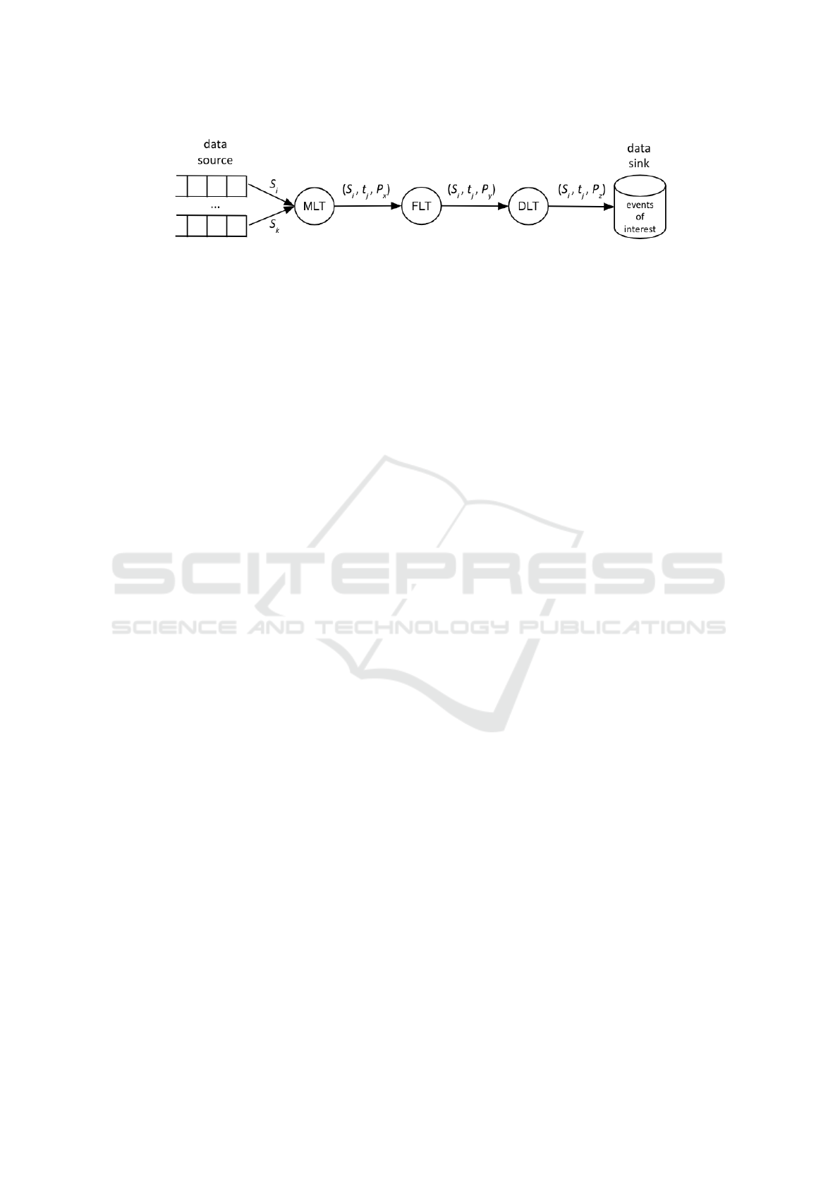
Figure 1: Application’s Workﬂow.

and the subset of idle nodes denoted as

IN = {e

∀i ∈ 1..β}, having λ + β = n (8)

The node selection algorithm is executed when

a new application submits its workﬂow to the sys-

tem. For a given workﬂow W

, the Orchestrator (a

component of MELINDA architecture) must choose

a set of edge nodes that can run the set of tasks

{MLT

, FLT

, DLT

}. An operator is the imple-

mentation of a processing task that runs on an edge

node. In this way, we have measurement level op-

erator (MLO), feature level operator (FLO), and de-

cision level operator (DLO). MLO and FLO opera-

tors perform deep learning (DL) tasks to detect and

identify objects of interest in messages IIM

i,t

, respec-

tively. So, to achieve low processing delays, these op-

erators run on edge nodes EN

⊆ EN equipped with

hardware accelerators optimized for neural networks.

The set of edge nodes EN

have different image

processing capacities measured in FPS. This capacity

is associated with the DL task running on a speciﬁc

node. Without loss of generality, we can assume that

every image in IIM

i,t

∀t = 0..∞ has the same resolu-

tion and takes the same processing time on a given

node e

. Therefore function Capacity(e

,task) re-

turns the capacity in FPS of node e

running task.

To guarantee this capacity, a node must only execute

one DL task per time. The reason for exclusive use

is that this type of processing generally consumes all

available hardware resources. The available idle ca-

pacity is given by function IC as the smallest value

between the sums of capacities of nodes U for MLT

and nodes V for FLT

, having U ∪V = IN. The for-

mal notation for function IC is given in equation (9)

where α and γ are the sizes of U and V , respectively,

and α + γ = β.

IC(W

) = min(

∑

i=1

Capacity(u

, MLT

∑

j=1

Capacity(v

, FLT

)) (9)

IC(W

) ≥ Flow(W

) (10)

The allocation of nodes should ensure that there

will be no bottlenecks in the workﬂow processing that

could lead to a steady increase in delays. If condition

(10) is not satisﬁed, then the workﬂow W

demands

processing capacity not available with the current set

of idle edge nodes, and the application’s request to

process W

will be declined. Otherwise, if (10) is true

then there are two sets U

⊆ U and V

⊆ V of edge

nodes that can process the workﬂow W

. In such a

case, the orchestrator allocates the edge nodes to exe-

cute workﬂow W

as E

= {U

∪V

}. Formally,

⊆ IN|E

= {E

MLO

∪ E

FLO

∪ E

DLO

} (11)

where E

MLO

, E

FLO

, and E

DLO

is the set of edge nodes

chosen to run MLT

, FLT

, and DLT

, respec-

tively.

3.2 Workload Distribution

Requesting the execution of a workﬂow to meet an ap-

plication requires the allocation of several edge nodes

to distribute the processing tasks of the associated

video streams. In this work, the node allocation rep-

resents a Deployment Plan. The allocation of image

processing tasks to nodes must meet the requirements

of low delay and maximum throughput, promoting

the usage of all the computational capacity of the allo-

cated nodes. According to (Dayarathna et al., 2016),

energy waste is mainly caused by nodes working in

idle state. Therefore, the ideal deployment plan is one

that respects the processing capacity of each node and

simultaneously processes an adequate number of im-

ages ﬂow for that set of allocated nodes.

The workﬂow deployment plan is a strategy for

creating a distributed processing infrastructure, sim-

ilar to a cluster. As in most cluster frameworks for

on-demand processing, a load balancing algorithm

is necessary to guarantee the best throughput. Only

when some MLO node produces an image of interest,

a FLO node processes this image. To prevent overload

in FLO nodes and avoid bottlenecks in the processing

ﬂow, we have developed a load balancing mechanism

for making the best possible usages of the available

resources at these nodes.

Our load balance approach uses the pattern pro-

ducer → worker → consumer of messages queue. We

created a microservice operator as a broker to control

Optimizing Resource Allocation in Edge-distributed Stream Processing

159

the load balancing. Figure 2 shows the workﬂow or-

ganization. MLO nodes are message producers, FLO

nodes are workers, and a DLO is the ﬁnal consumer

of the processing ﬂow. Since the broker and the DLO

operator’s tasks are lightweight processes compared

to those of the MLO and FLO operators, the broker

and DLO operator will be running on the same edge

node.

The broker uses two FIFO (First In, First Out)

message queues, one to receive all messages produced

by the MLO nodes (producers) and the other to for-

ward them to the ﬁnal consumer, the DLO node. The

producers feed the input queue, and the broker de-

livers the messages in the output queue to the con-

sumer using the PUSH-PULL messaging pattern. The

broker’s communication with workers is through the

REQUEST-REPLY pattern. In this case, the broker is

a client of the workers’ processing microservice, re-

questing the messages in the input queue and putting

the replies in the output queue. As the worker nodes

can have different processing capacities, the process-

ing of a message in a given node cannot delay pro-

cessing the next message in the queue. Thus, we use

the thread-based parallelism technique to treat the var-

ious messages in the input queue. There will be one

thread to communicate with each worker node. The

thread that connects to a fast worker will have its re-

ply before the others so that it will be able to read

and forward more messages than a thread with that

slower node. We detail the load balance algorithm in

(Rocha Neto et al., 2021).

4 THE RESOURCE ALLOCATION

ALGORITHM

This Section presents our algorithm to select nodes

to execute an image processing workﬂow denoted as

Flow(W

). This algorithm decides which nodes allo-

cate to run a workﬂow task (MLT or FLT) with the

lowest operational cost while respecting each node’s

limitations. We called a solution K

task

any set of

nodes e

∈ IN that can run task attending the workﬂow

demand Flow(W

). The set of all available nodes that

can run task is a solution, but this solution is probably

the most costly since it uses all disengaged resources.

Thus, we have an optimization problem to ﬁnd nodes

with the lowest operational cost to meet the workﬂow

processing capacity demand. Our objective function

is to minimize resource allocation costs, and our con-

straint is the sum of nodes’ processing capacity being

greater or equal to the workﬂow demand.

We deﬁne some metrics to evaluate node re-

sources. Regarding the latency, we considered the

processing and network delays. Using hardware

accelerators for neural networks, edge nodes can

achieve processing latency near-equivalent to cloud-

hosted nodes. Besides, the edge nodes’ network-

proximity with data source (sensors) tends to gener-

ate less transmission delays compared to nodes on the

cloud, compensating the longer processing delay. The

processing capacity c

of node e

to execute a task is

deﬁned as

= Capacity(e

,task),

∀e

∈ EN

,task ∈ {MLT, FLT } (12)

that informs the number of frames per second e

can

process for that task. For example, a node that can

process 20 FPS has a processing delay of 1/20 =

0.050, i.e., 50 ms to process each image.

To measure the network latency of a processor e

we deﬁne l

= Latency(e

, e

), ∀e

, e

∈ EN

(13)

where e

is the input data source node for e

. This

function checks how much time (in milliseconds) it

takes a message hop from e

to e

We deﬁne function Energy(e

,task) to measure e

the energy consumption in Watt per FPS for running

task. Hence,

= Energy(e

,task),

∀e

∈ EN

,task ∈ {MLT, FLT } (14)

is the variable to denote this consumption.

Function Availability(e

) calculates the availabil-

ity a

of a node e

. This function returns the ratio of

the up (available) time to the aggregated values of up

and down (not available) time, i.e.,

:: uptime

:: uptime + e

:: downtime

, ∀e

∈ EN (15)

where 0 ≤ a

≤ 1 and a

= 1 means e

was available

100% of the time. The cluster availability (CA) which

all nodes work in parallel (Tsai and Sang, 2010) is

deﬁned as

CA = 1 −

∏

i=1

(1 − a

) (16)

4.1 Objective Function

The proposed algorithm aims to select a set of nodes

with sufﬁcient capacity to process a workﬂow with

minimal cost. The cost is determined by capacity

waste (exceeding the workﬂow demand), network la-

tency from the input data source to the node, node en-

ergy consumption to process the messages, and node

unavailability. The unavailability is the complement

WEBIST 2021 - 17th International Conference on Web Information Systems and Technologies

160

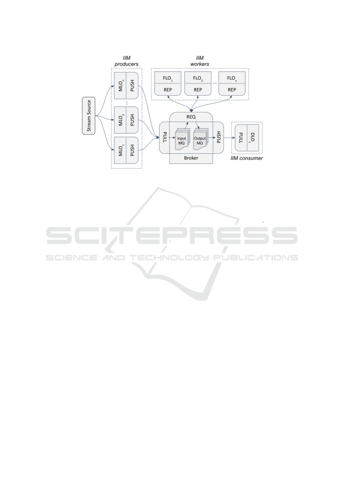
Figure 2: Workload distribution (Rocha Neto et al., 2021).

of the availability. Based on these criteria, equation

(17) provides our objective function for solving the

node allocation problem. We aim to achieve the low-

est operational cost (OC) as long as the nodes’ pro-

cessing capacity is sufﬁcient to handle a workﬂow.

minimize OC = A(

∑

− Flow(W

)) +

B(max(l

)) +C(

∑

) +

∏

(1 − a

))

subject to

∑

≥ Flow(W

) (17)

where

(

1, if e

is selected, ∀e

∈ IN ∧ c

> 0

0, otherwise

A, B, C, and D are coefﬁcients that represent the

unit costs of each metric evaluated to meet the appli-

cation’s QoS requirements. Coefﬁcient A deﬁnes the

cost for wasted capacity when the aggregate capac-

ity of selected nodes exceeds the capacity demanded

by the workﬂow. B, C, and D represent the costs for

network latency, energy consumption, and cluster un-

availability, respectively.

4.2 Optimizing Nodes Selection

To optimize the resource allocation choosing the best

solution, we have to deﬁne a brute-force search that

consists of systematically enumerating all possible

candidates for the solution and checking whether each

candidate satisﬁes the problem’s statement (equation

(17)). Thus, we developed an algorithm consisting

of two functions: (i) ﬁrst, it returns subsets of nodes

(combinations as candidate solutions) attending the

objective function constraint; (ii) for each subset (can-

didate), it calculates OC and returns the solution that

has the lowest cost.

Algorithm 1 represents the step (i) creating func-

tion Solutions that returns a set of nodes subsets that

can meet the workﬂow demand ( f ps

demand) as can-

didate solutions. First, the set of nodes is sorted ac-

cording to their processing capacity (line 2). Two

loops will then evaluate the combinations of a given

node (pivot) with the following nodes in decreasing

order of capacity until the sum of capacity is greater

than or equal to the requested capacity (lines 5–22).

If pivot capacity is equal to or greater than the work-

ﬂow demand (line 8), this node itself is a solution.

Otherwise, we test adding the capacity of the follow-

ing nodes (lines 11–20). We obtain a solution when

the added capacity is sufﬁcient (line 13). Still, the last

veriﬁed node i is not inserted in the partial variable

(lines 14–15), allowing to check other nodes in the

sequence that can ﬁt the remaining capacity.

Step (ii) is performed by function SelectNodes in

Algorithm 2. Its parameters are: IN is the list of idle

nodes; T is the image processing task (MLT or FLT)

the nodes will execute; F is the workﬂow demand

in FPS; IDS is the input data source to calculate the

transmission latency; and A, B, C, and D are weights

deﬁned according to the priority given by the appli-

cation to the different QoS parameters. After call-

ing function Solutions, this algorithm checks the cost

of each solution and selects the one with the lowest

value.

While a brute-force search is simple to implement

and will always ﬁnd a solution if it exists, its cost

is proportional to the number of candidate solutions,

which in our case tends to overgrow as the quantity of

Optimizing Resource Allocation in Edge-distributed Stream Processing

161

1 Function Solutions(nodes, f ps demand)

2 nodes ← sorted(nodes, key=c,

reverse=True)

3 solutions ←

4 k ← length(nodes)

5 for pivot ← 1 to k do

6 sumcap ← nodes[pivot] :: c

7 partial ← {nodes[pivot]}

8 if sumcap ≥ f ps demand then

9 solutions ← solutions ∪ partial

10 else

11 for i ← pivot + 1 to k do

12 cap ← sumcap + nodes[i] :: c

13 if cap ≥ f ps demand then

14 solution ←

partial ∪ {nodes[i]}

15 solutions ←

solutions ∪ solution

16 else

17 sumcap += nodes[i] :: c

18 partial ←

partial ∪ {nodes[i]}

19 return solutions

Algorithm 1: Selecting candidate solutions.

nodes increases. Algorithm 1 has an asymptotic

computational complexity of O(n log n) + O(n

O(n log n) is associated with the process of sorting

the nodes list (line 2), and O(n

) the two for-loop

to create the solutions space (lines 5–22). Generally,

heuristic algorithms are asymptotically better than ex-

act algorithms like this one, but they do not always

guarantee the best solution. As the number of nodes

tends to be limited, we can assume that our solution

has an acceptable computational time. For example,

considering a realistic scenario with 80 nodes avail-

able for processing, the algorithm took just 1.2 sec-

onds running on a Raspberry Pi 4 (4GB RAM) to

yield all workﬂows’ set of nodes to meet the given

application demand. The ﬁrst workﬂow arrangement,

which has all 80 nodes available, had 1,617 candidate

solutions.

5 EVALUATION

To evaluate the performance of MELINDA architec-

ture, we developed an intelligent application to assess

the processing time of running deep learning algo-

rithms on edge nodes (Rocha Neto et al., 2021). The

processing times were analyzed using real edge de-

vices equipped with accelerators for neural networks.

Once obtaining the operators’ processing times, we

1 Function

SelectNodes(IN, task, F, IDS, A, B,C, D)

2 nodes ← {e

..e

}, ∀e

∈

IN ∧Capacity(e

,task) > 0

3 K

task

← Solutions(nodes, F)

4 if length(K

task

) > 0 then

5 best cost ← ∞

6 best sol ← 0

7 for j ← 1 to length(K

task

), ∀e

∈ K

task

8 c

= Capacity(e

,task)

9 l

= Latency(IDS, e

)

10 w

= Energy(e

,task)

11 a

= Availability(e

)

12 cost ←

∑

) − F) + B(max(l

)) +

∑

) + D(

∏

(1 − a

))

13 if cost < best cost then

14 best cost ← cost

15 best sol ← j

16 return K

task

[best sol]

17 else

18 return

Algorithm 2: Selecting the best candidate.

used them in the YAFS simulator (Lera et al., 2019)

to scale up for a scenario with dozens of cameras and

processing nodes. With this simulator, we could eval-

uate MELINDA procedures meeting high-throughput

requirements in video analytics on the edge tier. The

scenario used as a running example consists of an

intelligent building with cameras scattered in open

spaces monitoring circulation. Edge nodes are in the

same camera’s network and equipped with hardware

accelerators for Edge AI (Lee et al., 2018). The re-

source allocation algorithm decides which nodes al-

locate to run a workﬂow task (MLT or FLT) with the

lowest operational cost while respecting each node’s

limitations. Although the application domain is im-

age processing in edge devices with DL accelerators,

this algorithm can be applied to any distributed pro-

cessing application running on nodes with different

processing capacities.

To assess our algorithm’s ability to choose nodes

with sufﬁcient capacity to process an application

workﬂow, we evaluated its performance by analyzing

two aspects: (i) its ability for choosing the combi-

nation of nodes with the lowest operational cost to

attend a workﬂow; and (ii) its skill to arrange more

workﬂows with the same set of available nodes. We

run a set of experiments that vary the nodes’ features

(processing capacity, communication latency from

data source, energy consumption, and node availabil-

WEBIST 2021 - 17th International Conference on Web Information Systems and Technologies

162

ity) for assessing each of these two aspects. We com-

pared the results with three well-known resource allo-

cation algorithms: ﬁrst-ﬁt, best-ﬁt, and worst-ﬁt. We

have not compared our algorithm with other works

(including some described in Section 6) because we

have not found a similar algorithm that jointly uses

the same metrics, thus preventing a fair compari-

son. Energy consumption and availability, for ex-

ample, are generally not considered in task place-

ment approaches as they historically run in powerful

and high-reliability environments, as is the case with

cloud data centers.

As algorithms’ data input, the features of each

node are in a tuple: (capacity in FPS, latency in ms,

energy in Watts / FPS, availability in percentage). The

tuples of all nodes are in a non-ordered array. The al-

gorithms’ objective is to select a set of nodes in which

the sum of processing capacity is greater or equal to

the workﬂow demand. In the ﬁrst-ﬁt approach, the al-

gorithm selects nodes as it reads the array until nodes’

capacity sum is equal to or greater than what is re-

quired by the workﬂow. Best-ﬁt and worst-ﬁt are sim-

ilar to ﬁrst-ﬁt; the difference is ordering the array by

the node capacity in descending (best-ﬁt) and ascend-

ing (worst-ﬁt) order before selecting each node. On

the other hand, our algorithm searches for all candi-

date solutions (any nodes combination attending the

constraint) and chooses the one with the lowest oper-

ational cost in terms of the best capacity ﬁt and QoS

criteria.

There is a direct relationship between process-

ing capacity and energy consumption. In our exper-

iments, the capacity (in FPS) and energy (in Watts /

FPS) data come from the evaluations in (Hernandez-

Juarez et al., 2016), where authors compared the

edge-based device NVIDIA Tegra X1 (10 Watts TDP)

with the powerful cloud-based NVIDIA Titan X (250

Watts TDP). Titan X achieved 3.54 FPS / Watt,

while Tegra X1 obtained 8.12 FPS / Watt. We ap-

plied these relations (inverting to Watts / FPS) in

our data array and vary the capacity per energy con-

sumption proportionally. Latency (in milliseconds)

and availability (uptime percentage) data are ran-

dom but based on our experiments using edge and

cloud nodes (Rocha Neto et al., 2021). The simula-

tion testbed used in these experiments is available in

https://github.com/aluiziorocha/MELINDA.

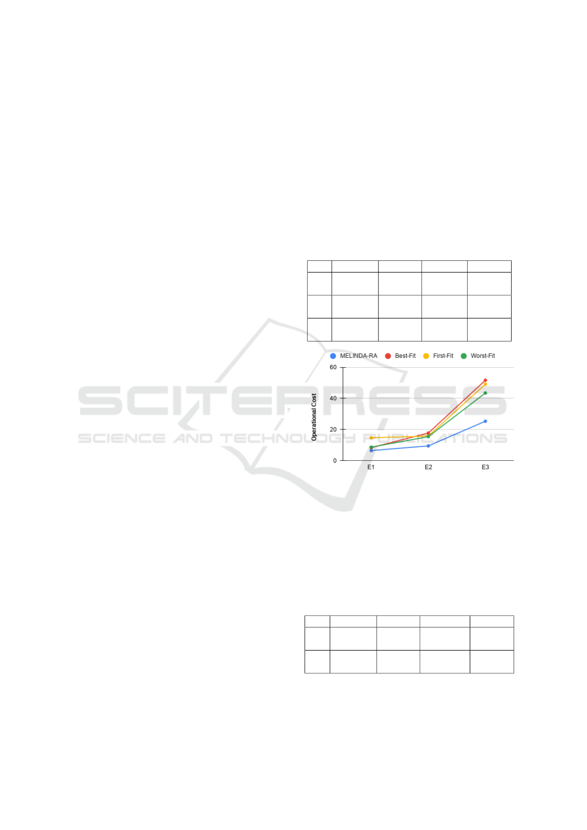
We performed three experiments (E1 to E3) to

evaluate the aspect (i) for each algorithm with dif-

ferent node sets. Each experiment represents a sce-

nario with varying degrees of node heterogeneity. Ta-

ble 1 shows the data for twenty nodes used in each

experiment, ranging from low (E1) to high (E3) de-

gree of heterogeneity. SD is the standard deviation,

i.e., the variation or dispersion of the set of val-

ues. In each experiment, the node allocation algo-

rithm should choose a set of nodes that could pro-

cess a workﬂow with a demand of 200 FPS. Fig-

ure 3 presents the operational cost calculated for

each algorithm and experiment. We named our al-

gorithm MELINDA-RA. As the nodes’ heterogene-

ity increases, MELINDA-RA becomes more efﬁcient

since it ﬁnds the nodes whose capacities best ﬁt the

remaining total. The other algorithms tend to choose

nodes whose capacity is much greater or lower than

that needed to meet the demand.

Table 1: Node heterogeneity in three experiments.

Capacity Latency Energy Availab.

E1 25 - 35 2 - 6 2.5 - 3.5 0.8 - 0.9

SD 3.753 1.352 0.375 0.02961

E2 20 - 40 2 - 10 3.1 - 6.0 0.6 - 0.9

SD 6.087 2.495 0.913 0.09324

E3 10 - 90 2 - 70 3.9 - 27.0 0.2 - 0.9

SD 25.761 21.597 7.728 0.17961

Figure 3: Operational cost for each method of allocating

nodes.

To evaluate the operational cost of edge, cloud,

and hybrid solutions, we also conducted some alloca-

tion tests in three scenarios: all nodes are edge de-

vices, all nodes are cloud computers and a mix of

both. Table 2 presents the data for twenty edge nodes

and twenty cloud nodes used in these tests, in which

the processing capacity demand is also 200 FPS.

Table 2: Edge and cloud nodes data.

Capacity Latency Energy Availab.

Ed. 25 - 35 2 - 6 3.1 - 4.3 0.7 - 0.8

SD 4.069 1.108 0.502 0.03194

Cl. 80 - 90 60 - 70 22.5 - 25.5 0.8 - 0.9

SD 2.555 2.937 0.721 0.02834

Figure 4 shows the maximum latency from the in-

put data source to the processing node in the cluster.

Solutions with only edge nodes are the ones that ob-

Optimizing Resource Allocation in Edge-distributed Stream Processing

163

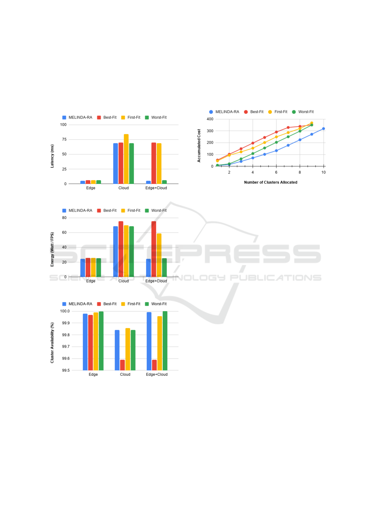
tain the lowest latency since the processors are close

to the data sources - the sensors. Figure 5 shows the

cluster’s total energy consumption by each method,

delivering the best results for the edge node solutions.

Figure 6 presents the availability of each cluster of

nodes. A more signiﬁcant number of edge nodes out-

performs the better availability of fewer nodes cloud.

Figure 4: Comparing latency using edge and cloud nodes.

Figure 5: Energy consumption comparison.

Figure 6: Cluster availability for edge and cloud nodes.

Finally, we evaluate the aspect (ii) related to

allocating the largest number of workﬂows with

the same set of available nodes. The most efﬁcient

algorithm is the one that distributes more workﬂows

and leaves fewer idle nodes. For this test, we used

the forty nodes’ hybrid solution in Table 2 with a

total processing capacity of 2,293 FPS. Then we ran

the algorithms to allocate the maximum number of

clusters, each one demanding 200 FPS for processing.

Figure 7 shows the accumulated cost for the number

of sets given. MELINDA-RA was the only one that

managed to allocate ten groups using all available

nodes. The other algorithms left nodes since their

processing capacity sum did not reach 200 FPS.

Figure 7: Allocating clusters with all available nodes.

6 RELATED WORK

In this Section, we present works dealing with dis-

tributed data stream processing in heterogeneous en-

vironments (Lahmar and Boukadi, 2020). The main

goal in most work is assigning nodes to meet a pro-

cessing demand imposed by a data stream. Amaras-

inghe et al., (Amarasinghe et al., 2018) proposes an

optimization framework that models the placement

scenario of data stream processing applications as

a constraint satisfaction problem (CSP). The frame-

work chooses the edge and cloud nodes to process the

data stream, considering nodes’ combination to min-

imize energy consumption and network latency. Al-

though the work considers edge and cloud nodes, the

lack of availability requirement, as a node choice al-

gorithm parameter, may make the solution unfeasible

in scenarios where some nodes may have a low degree

of availability.

Ghosh and Simmhan (Ghosh and Simmhan, 2018)

propose a genetic algorithm for distributing event-

based analytics tasks across edge and Cloud resources

to support IoT applications. They tacked the distribu-

tion of tasks as a constrained optimization problem.

The objective function was to minimize the end-to-

end processing latency regarding the constraints of

throughput capacity, bandwidth and latency limits of

the network, and energy capacity of the edge devices.

The authors modeled the placement strategy so that

every sink node is on the cloud, making the solution

unfeasible for some scenarios where the result of pro-

cessing a stream needs to be sent to an end-device at

the network edge. Moreover, the work does not con-

WEBIST 2021 - 17th International Conference on Web Information Systems and Technologies

164

sider availability as a constraint when choosing nodes.

Zeng et al. (Zeng et al., 2016) formulated the task

allocation and completion time minimization problem

as a Mixed-Integer Nonlinear Programming Problem

(MINLP). The main goal is to minimize the com-

pletion time of tasks distributing them between edge

nodes and end devices (clients) regarding load bal-

ancing. Some tasks are processed on clients for faster

response time. They proposed a heuristic algorithm

based on the MINLP formulation to minimize the

computation, transmission, and I/O time related to

the tasks’ execution, disregarding other QoS require-

ments such as availability and energy consumption.

In (Yang et al., 2020), authors propose an adaptive

multi-objective optimization task scheduling method

where the total execution time and the task resource

cost in the fog network are taken as the optimiza-

tion target of resource allocation. However, the op-

erational cost related to using the set of edge nodes

is calculated using just one QoS requirement. There-

fore, it can not effectively meet the multi-objective

requirements in real scenarios. Conversely, our pro-

posal considers four QoS requirements to derive the

operational cost. We also believe node availability is

an essential factor in node choice since edge/fog net-

works can suffer unpredictable instability.

Deng et al. (Deng et al., 2020) presents two algo-

rithms and a model for video analysis task allocation

in the mobile edge computing environment. The ﬁrst

one is a multi-round allocation algorithm based on

Exponential Moving Average (EMA) prediction used

when historical data cannot be obtained. On the other

hand, when long-term historical data is available, a

task online assignment algorithm is used based on the

reinforcement learning method (Q learning). In this

work, the available resources and capabilities of edge

nodes are not known a priori. Therefore the algo-

rithms need to estimate the capacities of edge nodes

to assign appropriate workload to them. Unlike our

approach, operational cost is deﬁned as cost per unit

of time, and the resource allocation algorithm does

not consider the availability and energy consumption

of nodes.

7 CONCLUSIONS

This paper presented an algorithm to allocate a set of

nodes for data streams distributed processing. The

algorithm performs an exhaustive search for the best

nodes combination considering the QoS requirements

communication latency from the data source, energy

consumption, and cluster availability. We evaluated

the algorithm with well-known methods of resource

allocation, and it achieved the best results always. We

also compared the choice of a set of edge nodes with

one of the cloud nodes. The edge set had several ad-

vantages, including better availability of the cluster by

having more nodes available.

As future work, we intend to improve the worker

nodes allocation process since the arrival of an image

of interest to this node depends on the device sensor’s

events. Even applying the worker task’s reuse as a

shareable Intelligence Service, their idleness can be

relatively high. Thus, the ideal solution would be to

predict events on each sensor according to their his-

tory within a time window. In this context, a promis-

ing approach is machine learning techniques for pat-

tern recognition in time-series data. With each camera

stream event pattern represented as a time window,

it is possible to predict the event rate and adjust the

number of workers accordingly.

Finally, advances in edge computing devices’ de-

velopment have made them smaller, more powerful,

and less energy-consuming. Besides, such devices’

collaboration has shown to be a promising approach

to overcome their limitations and achieve results sim-

ilar to the powerful processing nodes in the cloud.

ACKNOWLEDGEMENTS

This work is partially funded by CNPq (grant number

308274/2016-4) and by FAPESP (grant 2015/24144-

7). Professors Thais Batista, Flavia Delicato, and

Paulo Pires are CNPq Fellows.

REFERENCES

Amarasinghe, G., de Assunc¸

ao, M. D., Harwood, A., and

Karunasekera, S. (2018). A data stream processing

optimisation framework for edge computing applica-

tions. In 2018 IEEE 21st International Symposium

on Real-Time Distributed Computing (ISORC), pages

91–98, Singapore. IEEE.

Dautov, R., Distefano, S., Bruneo, D., Longo, F., Mer-

lino, G., and Puliaﬁto, A. (2017). Pushing intelli-

gence to the edge with a stream processing architec-

ture. In 2017 IEEE International Conference on Inter-

net of Things (iThings) and IEEE Green Computing

and Communications (GreenCom) and IEEE Cyber,

Physical and Social Computing (CPSCom) and IEEE

Smart Data (SmartData), pages 792–799, Exeter, UK.

IEEE.

Dayarathna, M., Wen, Y., and Fan, R. (2016). Data center

energy consumption modeling: A survey. IEEE Com-

munications Surveys Tutorials, 18(1):732–794.

de Assunc¸

ao, M. D., Veith, A. D. S., and Buyya, R.

(2017). Resource elasticity for distributed data stream

Optimizing Resource Allocation in Edge-distributed Stream Processing

165

processing: A survey and future directions. CoRR,

abs/1709.01363.

Deng, X., Li, J., Liu, E., and Zhang, H. (2020). Task alloca-

tion algorithm and optimization model on edge collab-

oration. Journal of Systems Architecture, 110:101778.

Garcia Lopez, P., Montresor, A., Epema, D., Datta, A., Hi-

gashino, T., Iamnitchi, A., Barcellos, M., Felber, P.,

and Riviere, E. (2015). Edge-centric computing: Vi-

sion and challenges. SIGCOMM Comput. Commun.

Rev., 45(5):37–42.

Ghosh, R. and Simmhan, Y. (2018). Distributed scheduling

of event analytics across edge and cloud. ACM Trans.

Cyber-Phys. Syst., 2(4).

Helal, S., Delicato, F. C., Margi, C. B., Misra, S., and

Endler, M. (2020). Challenges and opportunities for

data science and machine learning in iot systems - a

timely debate: Part 1. IEEE Internet of Things Maga-

zine, 4(1):2–8.

Hernandez-Juarez, D., Chac

on, A., Espinosa, A., V

azquez,

D., Moure, J., and L

opez, A. (2016). Embedded real-

time stereo estimation via semi-global matching on

the gpu. Procedia Computer Science, 80:143–153.

Huh, J.-H. and Seo, Y.-S. (2019). Understanding edge com-

puting: Engineering evolution with artiﬁcial intelli-

gence. IEEE Access, 7:164229–164245.

Lahmar, I. B. and Boukadi, K. (2020). Resource alloca-

tion in fog computing: A systematic mapping study.

In 2020 Fifth International Conference on Fog and

Mobile Edge Computing (FMEC), pages 86–93, Paris,

France. IEEE.

Lee, Y.-L., Tsung, P.-K., and Wu, M. (2018). Techology

trend of edge ai. In 2018 International Symposium on

VLSI Design, Automation and Test (VLSI-DAT), pages

1–2.

Lera, I., Guerrero, C., and Juiz, C. (2019). Yafs: A simula-

tor for iot scenarios in fog computing. IEEE Access,

7:91745–91758.

Mohammadi, M., Al-Fuqaha, A., Sorour, S., and Guizani,

M. (2018). Deep learning for iot big data and stream-

ing analytics: A survey. IEEE Communications Sur-

veys Tutorials, 20:2923–2960.

Nakamura, E. F., Loureiro, A. A. F., and Frery, A. C.

(2007). Information fusion for wireless sensor net-

works: Methods, models, and classiﬁcations. ACM

Comput. Surv., 39(3):9–es.

Qiu, J., Wu, Q., Ding, G., Xu, Y., and Feng, S. (2016). A

survey of machine learning for big data processing.

EURASIP J. Adv. Sig. Proc., 2016:67.

Ramos, E., Morabito, R., and Kainulainen, J. (2019). Dis-

tributing intelligence to the edge and beyond [research

frontier]. IEEE Computational Intelligence Magazine,

14(4):65–92.

Rocha Neto, A., Silva, T. P., Batista, T., Delicato, F. C.,

Pires, P. F., and Lopes, F. (2021). Leveraging edge

intelligence for video analytics in smart city applica-

tions. Information, 12(1).

Rocha Neto, A., Silva, T. P., Batista, T. V., Delicato, F. C.,

Pires, P. F., and Lopes, F. (2020). An architecture for

distributed video stream processing in IoMT systems.

Open Journal of Internet Of Things (OJIOT), 6(1):89–

104.

oger, H. and Mayer, R. (2019). A comprehensive survey

on parallelization and elasticity in stream processing.

ACM Comput. Surv., 52(2).

Tocz

e, K. and Nadjm-Tehrani, S. (2018). A taxonomy for

management and optimization of multiple resources

in edge computing. CoRR, abs/1801.05610.

Tsai, D. and Sang, H. (2010). Constructing a risk

dependency-based availability model. In 44th Annual

2010 IEEE International Carnahan Conference on

Security Technology, pages 218–220, San Jose, CA,

USA. IEEE.

Valera, M. and Velastin, S. A. (2005). Intelligent distributed

surveillance systems: a review. IEE Proceedings - Vi-

sion, Image and Signal Processing, 152(2):192–204.

Yang, M., Ma, H., Wei, S., Zeng, Y., Chen, Y., and Hu,

Y. (2020). A multi-objective task scheduling method

for fog computing in cyber-physical-social services.

IEEE Access, 8:65085–65095.

Zeng, D., Gu, L., Guo, S., Cheng, Z., and Yu, S. (2016).

Joint optimization of task scheduling and image place-

ment in fog computing supported software-deﬁned

embedded system. IEEE Transactions on Computers,

65(12):3702–3712.

WEBIST 2021 - 17th International Conference on Web Information Systems and Technologies

166