
Exploring the Decision Tree Method for Detecting Cognitive States of
Operators
Hélène Unrein
1
, Benjamin Chateau
2
and Jean-Marc André
1
1
IMS – Cognitique UMR 5218, ENSC-Bordeaux INP, Université de Bordeaux, Talence, France
2
Centre Aquitain des Technologies de l’Informations et Electroniques, Talence, France
Keywords: Cognitive States, Engagement in the Driving Task, Hypovigilance, Cognitive Fatigue, Eye-tracking, CARt.
Abstract: This study aims to validate a construction methodology of a device able to estimate the cognitive state of an
operator in real time.
The SUaaVE project (SUpporting acceptance of automated VEhicle) studies the integration of an intelligent
assistant in a level 4 autonomous car. The aim of our work is to model the cognitive state of the driver in real
time and for all situations. The cognitive state is a natural state that alters or preserves the operator's ability to
process information and to act.
Based on a literature review we identified the cognitive functions used by the driver and the factors influencing
them. Different cognitive components emerged from this synthesis: engagement (Witmer & Singer, 1998),
fatigue (Marcora and al. 2009) and vigilance (Picot, 2009).
Eye-tracking is a technique used to determine the orientation of the gaze in a visual scene. According to the
literature the general dynamics of a visual behavior is characterized by metrics: number of fixations, duration
of fixation, gaze dispersion... These dynamics are altered unconsciously due to fatigue (Faber, Maurits, &
Lorist, 2012) or hypovigilance (De Gennaro et al., 2000, Bodala et al., 2016); and consciously due to
engagement in driving (Freydier et al., 2014; Neboit, 1982).
We carry out a phase of experimentation in a naturalistic situation (driving simulator) in order to collect data
for each cognitive state. Realistic scenarios are constructed to induce cognitive states. The model’s estimation
is compared to the real cognitive state of the driver measured by behavioral monitoring (eye-tracking).
The model is a CARt (Breiman & Ihaka, 1984) decision tree: Classification And Regression Trees. The CARt
aims at building a predictor. The interest is to facilitate the design of the tool as well as its future
implementation in real time. We illustrate the construction methodology with an example the results obtained.
1 RESEARCH PROBLEM
The SUaaVE project studies the integration of an
intelligent assistant in a level 4 autonomous car. This
assistant will provide a set of services to enhance the
user experience in the vehicle, based on of an
assessment of the driver state. In this context, the aim
of our work is to model the cognitive state of the
driver in real time and for all situations.
2 OUTLINE OF OBJECTIVES
This study aims to validate a device (ALFRED) able
to estimate the cognitive state of an operator.
The cognitive model we propose informs
ALFRED of the operator's state in real time. The
cognitive state is a natural state that alters or preserves
the operator's ability to process information and to
act. In real time and in a car cockpit, cognitive states
are difficult to observe. Their measurement/detection
is done in a dynamic, uncontrolled environment
(changing luminosity) which is limiting the use of
certain sensors. These constraints lead us to choose a
specific sensor and tolerant to the effect of the
environment: occulometry sensor.
The cognitive model we propose is based on
different dimensions: engagement (interest for the
road situation, Witmer & Singer, 1998),
hypovigilance (Picot, 2009), fatigue (Marcora et al.,
2009). Each dimension is discriminated by specific
210
Unrein, H., Chateau, B. and André, J.
Exploring the Decision Tree Method for Detecting Cognitive States of Operators.
DOI: 10.5220/0010712300003060
In Proceedings of the 5th International Conference on Computer-Human Interaction Research and Applications (CHIRA 2021), pages 210-218
ISBN: 978-989-758-538-8; ISSN: 2184-3244
Copyright
c
2021 by SCITEPRESS – Science and Technology Publications, Lda. All rights reserved

ocular behaviors, measurable with an eye-tracker
(fixations and saccades).
Each behavior must be coded and integrated into
the ALFRED cognitive module. To do so, it is
necessary to validate the instrumental efficiency of
the eye-tracking data processing for each of the 3
selected dimensions. The results will allow the
selection of the most interesting dimension(s) and
will guide the development of a real time data
processing solution.
3 BACKGROUND
3.1 Definition
A cognitive state is a psycho-physiological state that
alters or not the cognitive capacities of the operator.
A cognitive state is composed of a set of cognitive
dimensions: cognitive load, physical fatigue,
expertise in the task, attention, etc. Each cognitive
dimension has its own characteristics:
- Role: alert, maintenance, information collection.
- Mechanisms: different levels or phases
throughout the day/week/month; regulation by
positive or negative feedback, by reaction.
- Effects on the operator's cognitive capacities:
induced failures, maintained capacities.
In addition, the cognitive dimensions have
interactions between them. There are as many
cognitive states as there are possible crossings
between the different levels of the cognitive
dimensions.
3.2 Constraints
All sensors are not necessarily operational in our
context. Indeed, we are confronted with several
constraints :
- Tolerance to "noise": ability of an instrument to
provide a measurement resistant to undesirable
parameters (lighting variations...)
- Portability: ability to be easily transported
- Acceptability: degree of user's acceptance to wear
or use the measurement device.
- Ease of implementation: cost, complexity of
implementation.
According to the constraints, the sensor must be
portable, non-intrusive and noise tolerant. The
measurements of the dimensions are behavioral.
These measurements must have a sufficient level of
acceptability (non-intrusive) and noise tolerance. The
operator must not be interrupted.
All these constraints have reduced the field of
possibilities. The following cognitive dimensions
satisfy these constraints.
3.3 Cognitive Dimensions
Three cognitive states were identified in a literature
review:
Engagement in the driving task is a psychological
state. It is the consequence of focusing our energy and
attention on a coherent set of stimuli and related
events (Witmer & Singer, 1998).
Hypovigilance corresponds to the transition
between alertness and sleep during which the
organism's observation and analysis faculties are
reduced (Picot, 2009): decreased attention, increased
information processing and decision making time,
etc.
Cognitive fatigue is a psychological condition
caused by prolonged periods of demanding cognitive
activity (Marcora et al., 2009). Cognitive fatigue
decreases the individual's ability to perform a task by
altering states of alertness and focused attention
(Thiffault & Bergeron, 2003).
3.4 Ocular Behavior
Eye-tracking trajectories are composed of fixations
and saccades. When a human being focuses on a point
of interest, the gaze moves around this area (see
Figure 1). The eyes are always moving in our visual
environ-ment in order to allow an active vision of the
reality around us. This is why a fixation, when we
analyze an element, never has a single position of the
gaze.
Between two fixations, we make quick
movements called saccades. They allow us to position
our gaze on the object of interest.
Figure 1: Representations of gaze positions according to the
type of ocular event.
3.5 Eye-tracking
Interest of eye-tracking
Eye-tracking is a technique used to determine the
orientation of the gaze in a visual scene. According to
the literature the general dynamics of a visual
behavior is characterized by the following metrics:
number of fixations, duration of fixation, gaze
Exploring the Decision Tree Method for Detecting Cognitive States of Operators
211
dispersion, distance between two saccades, saccade
speed, saccade amplitude, and eye deflection angle.
These dynamics are altered unconsciously due to
fatigue (Faber, Maurits, & Lorist, 2012) or
hypovigilance (De Gennaro et al., 2000, Bodala et al.,
2016); and consciously due to engagement in driving
(Freydier et al., 2014; Neboit, 1982).
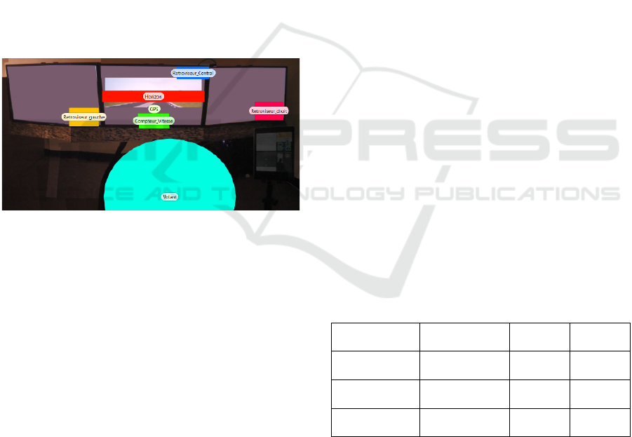
Area of Interest (AOI)
Eye-tracking allows us to identify the elements and
areas that the driver looks at. The areas of interest
(AOI) represent the regular fixation points of a driver
(Neboit, 1982 and Freydier, 2014) (Cf Figure 2):
- Interior and exterior mirrors - 3 AOI: "Left
mirror", "Right mirror", "Center mirror" ;
- Vehicle Controls - 2 AOI: "GPS", "Steering
Wheel" ;
- Speedometer - 1AOI: "Speedometer".
The fixations in the far forward area represent an
attention disengagement fixation area: 1 AOI -
"Horizon.
Figure 2: Spatial representation of the areas of interest on
the reference image of the participants' full visual field.
The cockpit areas do not change location despite
the movement of the vehicle. Their static position
allows for automated image processing to identify the
position of the gaze throughout the experiment. This
automated processing requires a reference image (see
Figure 2) where all the areas of interest are indicated.
4 METHODOLOGY
The instrumental validation regarding the detection of
the cognitive state is based on induction and
observation: induction of the operator's cognitive
state by the experimental conditions, observation of
the ocular behavior. The study of the cognitive model
is based on different realistic scenarios constructed to
induce cognitive states which will be detailed.
The induction was operationalized on the basis of
3 test scenarios of driving an autonomous vehicle in
a simulator, one scenario per induced cognitive
dimension: engagement, hypovigilance, fatigue. This
induction is based on the information provided by the
literature and the adapted environment.
The data associated with the cognitive states are
collected during experimental tests in simulation with
the objective of collecting oculometric data. The
objective is to associate each cognitive state of
interest with a typical visual behavior detectable by
the oculometric data.
4.1 Participants
40 participants were recruited. Thirty-three
participants completed the entire experiment.
Recruitment was done mostly by email via the
campus lists of the University of Talence at the
following institutions: IMS Laboratory, Bordeaux-
INP, INRIA, University of Bordeaux. All of the
volunteers were offered a 20 € gift card to participate
in this experiment. All gave free and informed
consent.
The inclusion criteria for the panel (see A.1)
targeted experienced participants, preferably with
regular driving experience. The native language must
be French to avoid bias in the understanding of the
questionnaires. The exclusion criteria (cf. A.2)
exclude participants with potential problems of
immersion in a virtual reality: epileptic,
claustrophobic, cybersickness, etc.
The initial sample included an equitable
distribution of gender and age. However, senior
adults are more susceptible to simulator sickness (a
syndrome closely related to motion sickness), making
recruitment more difficult. Table 1 shows the
complete study sample.
Table 1: Characteristics (age and gender) of participants.
Age / Sexe Man Woman Total
- 45 years old 21 8 29
+ 45 years old 3 1 4
Total 24 9 33
Our population is 27% female and 73% male,
with 88% 45 years old and 12% over 45. Our
population is essentially made of men under 45 years
old with a proportion of 64% against 9% of men over
45 years old; 24% of women under 45 years old and
3% of women over 45 years old.
CHIRA 2021 - 5th International Conference on Computer-Human Interaction Research and Applications
212

4.2 Material
4.2.1 Simulator
- A neutral and silent experiment room (about 8m²),
- Driving seat: ATGP Playseat,
- Logitech G27 driver's station with steering wheel,
pedals and gear shift lift,
- Computer with simulation software,
- Simulation software: A.V. Simulation (formerly
Oktal) SCANeR Studio™, version 1.8,
- Three high-resolution 32-inch screens (2560 x
1440 pixels). These screens have been aligned to
offer an immersion adapted to the 3D scene of the
simulation (alignment of lines crossing several
screens), and thus reduce the risk of
cybersickness.
4.2.2 Sensor
The eye-tracker used is a Tobii Pro Glasses 2
(200Hz): eye-tracker worn binocular. These eye-
trackers is worn by the operators as glasses. The
binocular eye-trackers is equipped with three
cameras: 2 cameras capture the images of the eyes
and one camera, called scene camera, captures the
visual field of the operator. The scene camera records
the video of the environment on which the fixations
will be affixed in order to visualize the visual
behavior. The horizontal field of view of the scene
camera is 60◦.
The glasses are connected to a recording unit via
a cable in Micro USB. With an autonomy of 105
minutes the storage media is equipped with an SD
card. The unit is connected to the local network via an
Ethernet cable.
4.3 Measurement
4.3.1 Independent Variables - Controlled
Cognitive states were considered known and
indicated in the data by the variable
"Characterization": a categorical variable with three
levels, 1 for engagement, 2 for hypovigilance and 3
for fatigue.
4.3.2 Dependent Variables – Observed
The values of the visual metrics depending on the
cognitive state are unknown. These are the dependent
variables of the model.
Each metric is represented by a numerical variable.
They are calculated thanks to the eye-tracker data:
position of the gaze in the experimental environment.
Eleven metrics have been identified through a
literature search (table 2). A metric is calculated over
a 20 second window. This window is sliding of one
second which makes 11 data per second.
Table 2: List of dependent variables calculated according to
the associated cognitive state.
Engagement
1
Hypovigilance² Fatigue
3
Fixation
frequency in AOI
Fixation
frequency in the
horizon
Fixation duration
in AOI
Gaze dispersion
Gaze dispersion
in AOI
Distance
between two
saccades
Saccade speed
Fixation frequency
Fixation duration
Eye deflection angle
Saccade speed
Saccade amplitude
1
Freydier and al., 2014; Neboit, 1982
² De Gennaro and al., 2000, Bodala and al., 2016
3
Silvagni and al., 2020; Yonggang Wang and Ma, 2018;
Hjälmdahl and al., 2017
4.3.3 Link between Test and Model
The final cognitive model can be written in the form
𝑌 ~ 𝛽
+𝛽
.𝑥
+⋯+𝛽
.𝑥
+𝜀.
The oculometric data or visual metrics are the
dependent variables of the experimental tests:
observed variables. In the final model they are the
input data: explicative variables 𝑥 explicatives,
independent variable of the model.
The known cognitive state is the independent
variable of the experimental tests: controlled variable.
In the final model it is the output data: explained
variable Y, dependent variable of the model.
4.4 Procedure
After a presentation of the study and a first
cybersickness questionnaire, the participant is
installed at the driving station. The experimenter
presents the controls and indicators of the dashboard,
then installs and calibrates the eyetracker. Then the
participant carries out the 4 driving scenarios: 1
familiarization scenario in autonomous and manual
mode, 3 tests in 100% autonomous. After each
scenario, the participant answers questionnaire
relating to the cybersickness (Kennedy et al. 1993). If
the cybersickness score is suitable (score below 8)
then the participant may continue. Before launching
the next scenario, the experimenter suggests taking a
break. Finally, the participant fills in the socio-
demographic questionnaire before being thanked.
Exploring the Decision Tree Method for Detecting Cognitive States of Operators
213

4.5 Scenario Setup
The participants' cognitive states are induced by the
experimental conditions: environment and cognitive
task. 4 test scenarios were constructed: (1)
Familiarization with the simulator and autonomous
mode; (2) Engagement phase; (3) Hypovigilance
phase; (4) Fatigue phase.
Familiarization with the simulator and
autonomous mode
This phase is necessary to avoid learning bias by
familiarizing the participant with the automatic car
controls and the virtual environment. It is carried out
before the experimental scenarios.
After explanations on how the simulator works,
the participants performes a driving task lasting
approximately 15 minutes. In this scenario, the
participants drive on all three types of roads for 5
minutes each: city, outskirts and motorway. On the
outskirts and the motorway participants are asked to
switch on/off the autonomous mode. Using the
manual mode allows the user to familiarize himself
with the simulator by transposing his driving
automatisms.
At the end of the training phase, the participant is
able to control the vehicle correctly. Getting back in
control, checking the deviation from the axis and
checking the indicators remains the usual three points
of difficulty.
Engagement phase
This phase has been designed to record the driver's
reference eye behavior while engaged in 100%
autonomous driving. The scenario presents a variety
of road situations and events: other cars, more or less
steep country roads, varied landscapes, etc.
Hypovigilance phase
Hypovigilance is characterized by a loss of attention
to elements of the situation. It is induced here by a
monotonous driving situation (McBain, 1970;
Wertheim, 1991), in which the user's attention is little
solicited by new events. This scenario is
characterized by the following parameters:
- A repetitive environment (Thiffault & Bergeron,
2003): flat terrain; the pines on each side of the
road at a frequency of 2 per second, at a speed of
80 km/h; the pines are visible up to the horizon.
- A 15-minute driving task poor in event. The driver
has to follow a lane at a constant speed (80 km/h),
without changing gears, changing lanes and
without using car features (e.g. turn signals,
mirrors).
- Few variations in road infrastructure (Larue et al.,
2011): no red lights, no stopping, little traffic; no
T or perpendicular bends, the road is essentially
straight with few curves.
Fatigue phase
The driving scenario is similar to that of the
engagement phase. The objective is not to observe
hypovigilance but a state of fatigue despite an
engaging environment. A constant cognitive load for
more than 10 minutes causes cognitive fatigue
(Borragán et al., 2016). Cognitive fatigue is induced
by performing a difficult n-back task for 15 minutes.
Once the 15 minutes of mental effort are passed, the
driver checks the trajectory of the car during the
remaining 5 minutes, as in the previous stage. This
makes it possible to collect ocular data on fatigue.
5 BEHAVIOUR PROCESSING
ALGORITHMS
5.1 Pre-Processing of Raw Data
Each cognitive dimension is discriminated by a set of
visual metrics calculated from the raw data. The
metrics are associated with areas of interest in the
environment. To calculate these metrics, several
processes are necessary. The first one consists in a
filter to detect fixations and saccades, the second one
in a mapping to detect events in the areas of interest.
The visual metrics are calculated on these mapped
data.
5.1.1 Raw Data
The output data of an eye-tracker is presented in an
Excel sheet with 200 observations per second. In
general, each observation is composed of:
- a timestamp: time in millisecond;
- the direction in x, y and z of the right and left eyes;
- the validity of the detection of the eyes position of
the gaze in x and y;
- the frame index of the closest video.
5.1.2 Filtered Data
The offline processing of the raw data is done by the
software associated with the eye-tracker: Tobii Pro
Lab. The processing is a classification filter for the
type of event associated with the gaze position:
fixation or saccade. The filter settings are the
following:
CHIRA 2021 - 5th International Conference on Computer-Human Interaction Research and Applications
214

Table 3: Value of the settings of the filter for the detection
of fixations and saccades.
Fixation-Saccade detection filter
settin
g
s
Parameter values
Max
g
a
p
len
g
th
(
ms
)
150
Noise reduction moving median,
window size
(
sam
p
les
)
:3
Velocity calculator - window length
(
ms
)
20
I-VT classifie
r
- Threshol
d
(
°/s
)
35
Merge adjacent fixation
- max time between fixations (ms)
- max angle
b
etween fixation (°)
true
60
0.25
Discard short fixation - Minimum
fixation duration
(
ms
)
200
The output data is called filtered data and is
associated with an image from the scene camera
video. The gaze position is superposed on this video
providing a clear replay of the participant's visual
trajectories. The filtered data are composed of :
- The position of the gaze: x,y;
- The index of the closest video frame;
- The type of event: fixation, saccade, unclassified;
- The duration of the event in milliseconds;
- The index of the type of eye movement: represents
the order in which an eye movement was
recorded. The index is an auto-incrementing
number starting with 1 for each eye event type.
5.1.3 Mapped Data
Offline processing of the filtered data is also done by
the Tobii Pro Lab software. The processing is a
mapping detecting the areas of interest in the video
images. The objective is to identify the events in the
areas of interest. The mapping is performed on a
reference image (see Figure 2). This reference image
includes all the areas of interest unlike the scene
camera which does not have a sufficient field of
view. The result of this processing is gaze data
mapped on this reference image. The mapped data is
composed of:
- The presence of the gaze or not in an area of
interest: 0 (absence) or 1 (presence). One
variable per area of interest;
- The coordinates of the eye position, x,y on the
reference image;
- Confidence score of the mapping: validity score
of the mapped gaze points;
- The type of event: fixation, saccade,
unclassified;
- The duration of the event in milliseconds;
- The index of the type of eye movement.
A selection of mapped data is applied including a
removal of bad mapped events and a removal of
outliers. The quality of the mapping is indicated by a
confidence score. If the confidence score is less than
0.4, the data is deleted. Beyond this threshold, the loss
of data is more than 20%. This adjustment is coherent
with respect to the literature (Lemercier and al., 2015;
Winn, Wendt, Koelewijn, & Kuchinsky, 2018).
Saccades not surrounded by fixation and far from the
mean visual field are suppressed. No interpolation
was done to avoid adding non-existent information
and altering the calculation of metrics.
5.2 Visual Metrics Calculation
Visual behavior metrics are calculated from the
mapped and corrected data. Our hypothesis is that the
metrics vary with the participant's cognitive state.
The calculated metrics are the dependent variables of
the experimental tests. They will be the inputs to our
detection model. Eleven metrics were identified as
markers of specific cognitive states (Table 2) :
Engagement: 3 discrete variables in the integer
space
1. Frequency of fixation in areas of interest;
2. Fixation frequency at the horizon.
The frequencies are the sum of the number of
fixations in the areas of interest over a 20 second
window.
3. Fixation duration in the areas of interest: average
duration of fixations in the areas of interest over a 20-
second window.
Hypovigilance: 4 continuous variables in the
space of positive reals
1. Dispersion of the gaze in the visual field;
2. Gaze dispersion in the areas of interest.
Dispersions are the average Q3-Q1 interquartile
range of the spatial distance between each gaze point
(in the AOI) and the median gaze point over a 20-
second window. 50% of the observations are
concentrated between Q1 and Q3.
4. Distance between two saccades: average of the
distances between the end of one saccade and the
beginning of another over a 20 second window.
5. Saccade speed: average speed of saccades over a
20-second window.
Cognitive fatigue: 5 variables
1. Fixation frequency: sum of the number of fixations
over a 20 second window; discrete variable in an
integer space.
Exploring the Decision Tree Method for Detecting Cognitive States of Operators
215

2. Fixation duration: average duration of fixations
over a 20-second window; discrete variable in an
integer space.
3. Eye deflection angle: average of the angle between
two vectors formed by the X and Y directions of the
eyes over a 20 second window; continuous variable
in positive real space.
4. Saccade speed: average speed of saccades over a
20-second window; continuous variable in positive
real space.
5. Saccade amplitude: average of the distances
between the beginning and the end of the same
saccade over a 20 second window; continuous
variable in the space of positive reals.
All metrics were calculated over the three phases
of the scenario: engagement, hypovigilance and
fatigue. Each metric is calculated over a 20-second
window. This 20 second window slides by one second
which makes 11 observations per second per phase
per participant.
It is necessary to know the behavior of the metric
on all phases to characterize differences between
phases.
6 FIRST RESULTS
The model is a CARt decision tree built on the data
set. The set of independent variables of an individual
classifies him in a cognitive state.
6.1 Method of Analysis
The Classification And Regression Trees - CARt
(Breiman & Ihaka, 1984) are supervised learning
methods. The tree tries to solve a classification
problem. Mathematically speaking, the method
performs a binary recursive partitioning by local
maximization of the heterogeneity decrease.
The CARt aims at building a predictor: predicting
the values taken by our dependent variable Y
(cognitive state) as a function of the independent
variables X (visual metrics).
This prediction is based on a tree where each node
corresponds to a decision about the Y value. This
decision is made according to the value of one of the
Xs. At each node, the tree splits the data of the current
node into two child nodes. The individuals are
divided into the two most homogeneous subsets (Gini
diversity index) possible in terms of Y. The first
nodes use the most important variables. Not all
metrics are necessarily used in the construction of the
tree. A significant variable is not used if another is
highly correlated with it. The terminal leaves give the
predictions of Y.
The independent and dependent variables can be
quantitative or qualitative. Here the independent
variables are quantitative. The dependent variable is
categorical at three levels: 1 for engagement, 2 for
hypovigilance and 3 for fatigue.
6.2 Dataset
3 recordings corresponding to the 3 tests scenarios are
associated with each participant. The scenarios are
divided into two periods. The first provokes the
desired cognitive state, which is observed during the
second. The first period provokes a cognitive state
that is under-adjusted due to the chosen
environmental conditions. The second period is the
moment when the participant is actually in the desired
cognitive state. The learning phase is not included in
these two periods. The periods of interest occur at
different times (minutes) depending on the scenario:
- Scenario 1: observation of an engaged
participant during the next 3 minutes of the
scenario.
- Scenario 2: induction of hypovigilance during
the first 15 minutes of the scenario; observation
of a hypovigilant participant during the next 3
minutes of the scenario.
- Scenario 3: Induction of fatigue during the first
15 minutes of the scenario; observation of a tired
participant during the next 3 minutes of the
scenario.
Metrics calculation are done on the second
periods of the scenarios. A data is composed of the
value of the 11 metrics for one second for a
participant. This makes a total of 17,820 data: 33
participants, 3 test scenarios, 180 seconds. The data
does not have to be normalized. All these data are the
dataset for the construction of the CARt.
6.3 Decisional Tree
The decision tree (Figure 3) was built with the rpart
package. First, the tree was built on all the data with
the tree building function rpart() of the package. We
keep the default parameters. The learning error is
48%.
In figure 3, we can read the tree as follows. At the
root of the tree there is a node that splits into two
branches: branch 1 on the left and branch 2 on the
right. Branch 1 corresponds to the participants' data
such that the “number of fixations on the horizon”
exceeds the threshold of 11.5 fixations / 20 seconds.
CHIRA 2021 - 5th International Conference on Computer-Human Interaction Research and Applications
216
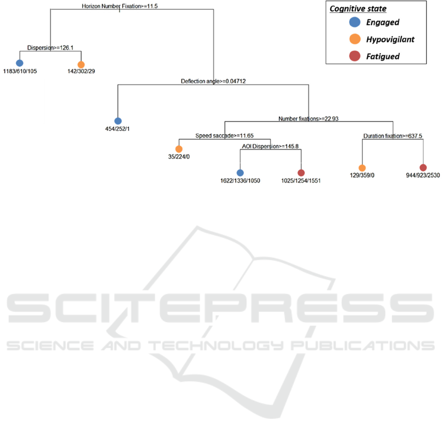
Figure 3: First version of the CARt for the detection of the cognitive state of the operator, construction of the data set.
Branch 1 splits into two end leaves: leaf 1 on the
left and leaf 2 on the right. Leaf 1 corresponds to the
data of participants such that the "gaze dispersion"
exceeds the threshold of 126.1 pixels / 20 seconds. In
this leaf 1 the cognitive state detected is engagement.
The 3 indicators under the end leaf indicate the
distribution of the participants' data classified in this
leaf according to their actual cognitive state: engaged/
hypovigilant / tired.
1183 data from engaged participants are classified
as engaged; 610 data from hypovigilant participants
are classified as engaged; 105 data from tired
participants are classified as engaged. Here the
number of correct classifications prevails by 62%.
Leaf 2 corresponds to the data from participants
such that the gaze dispersion does not exceed the
threshold of 126.1 pixels / 20 seconds. In this leaf 2
the cognitive state detected is hypovigilance. 142 data
from engaged participants were classified as
hypovigilant; 302 data from hypovigilant participants
are correctly classified as hypovigilant; 29 data from
fatigued participants are classified as hypovigilant.
The number of correct classifications prevailed by
63%.
The determination of the operator's cognitive state
stops when the reading of the model results in a
terminal leaf. The model always determines an
output. If the operator is not in one of these three
states the model returns the closest cognitive state.
6.4 Predictive Quality Validation
The cross-validation method (Mosteller & Tukey,
1968) partitions the data into 3 subsets. Each subset
is successively used as a test sample, the rest as a
learning sample: 2/3 for learning and 1/3 for testing.
The tree, our estimator, is computed on the training
data. The prediction error is calculated on the test
data. At the end of the procedure, we obtain 3
performance scores: percentage of error. The mean
and the standard deviation of the 3 scores respectively
estimate the percentage of error and the variance of
the validation performance.
The three performance scores obtained are: 65%,
67% and 67%. This makes an average of 66% and a
standard deviation of 0.0011. We find that, as it
stands, the model does not perform well enough to
accurately predict the values of the cognitive state
variable Y.
In order to improve our model, as we explain in
paragraph 7, a descriptive study of the data is in
progress. Our objective is to identify possible outliers
that would decrease the performance of the model.
7 EXPECTED OUTCOME
The objective of our approach is the construction of
an efficient detector tree with a test error of about
20%.
Analyses are in progress and will allow the
realization of a satisfactory predictive tree. New data
sets are built from existing data such as the
exploration of the variations of visual metrics. The
variations are calculated in points and in percentages
for each individual. If the percentage variations are
significant, the intra-individual difference is
important. The realization of a single tree per operator
is considered.
Automatic classification of a group of individuals
for each cognitive state is planned. The objective is to
Exploring the Decision Tree Method for Detecting Cognitive States of Operators
217

identify groups of individuals and operator profiles.
The hypothesis is that the inter-individual difference
is too important for the realization of a general model
for all operators.
A sub-model of fatigue will be developed to
enable the concomitance of several cognitive states to
be addressed.
8 CONCLUSION
Our research aims at defining a method to design a
predictor of the cognitive state of operators based on
their visual behavior. The interest is to facilitate the
design of the tool as well as its future implementation
in real time. In this paper, we present the
methodology for the conception of the predictor and
illustrate with an example the results obtained. Our
objective is twofold. The first one is the development
of a performant predictor; the second one is the
application of this method on future eye-tracking
data. In the second case, it will allow the
improvement of the predictor by the integration of
new data for the detection of other cognitive states:
physical fatigue, mental load, attention.
REFERENCES
Bodala, I. P., Li, J., Thakor, N. V., & Al-Nashash, H.
(2016). EEG and eye tracking demonstrate vigilance
enhancement with challenge integration. Frontiers in
human neuroscience, 10, 273.
Borragán, G., Slama, H., Destrebecqz, A., & Peigneux, P.
(2016). Cognitive fatigue facilitates procedural sequence
learning. Frontiers in human neuroscience, 10, 86.
Breiman, L., & Ihaka, R. (1984). Nonlinear discriminant
analysis via scaling and ACE. Department of Statistics,
University of California.
De Gennaro, L., Ferrara, M., Urbani, L., & Bertini, M.
(2000). Oculomotor impairment after 1 night of total
sleep deprivation : A dissociation between measures of
speed and accuracy. Clinical Neurophysiology,
111(10), 1771-1778.
Faber, L. G., Maurits, N. M., & Lorist, M. M. (2012).
Mental Fatigue Affects Visual Selective Attention.
PLOS ONE, 7(10), e48073. https://doi.org/10.1371/
journal.pone.0048073
Freydier, C., Berthelon, C., Bastien-Toniazzo, M., &
Gineyt, G. (2014). Divided attention in young drivers
under the influence of alcohol. Journal of safety
research, 49, 13. e1-18.
Kennedy, R. S., Lane, N. E., Berbaum, K. S., & Lilienthal,
M. G. (1993). Simulator sickness questionnaire : An
enhanced method for quantifying simulator sickness.
The international journal of aviation psychology, 3(3),
203-220.
Larue, G. S., Rakotonirainy, A., & Pettitt, A. N. (2011).
Driving performance impairments due to hypovigilance
on monotonous roads. Accident Analysis & Prevention,
43(6), 2037-2046. https://doi.org/10.1016/j.aap.20
11.05.023
Lemercier, A., Guillot, G., Courcoux, P., Garrel, C.,
Baccino, T., & Schlich, P. (2014). Pupillometry of
taste : Methodological guide–from acquisition to data
processing-and toolbox for MATLAB. Quantitative
Methods for Psychology, 10(2), 179-195.
Marcora, S. M., Staiano, W., & Manning, V. (2009). Mental
fatigue impairs physical performance in humans. J.
Appl. Physiol.
McBain, W. N. (1970). Arousal, monotony, and accidents
in line driving. Journal of Applied Psychology, 54(6),
509.
Mosteller, F., & Tukey, J. W. (1968). Data analysis,
including statistics. Handbook of social psychology, 2,
80-203.
Neboit, M. (1982). L’exploration visuelle du conducteur :
Rôle de l’apprentissage et de l’expérience. CAH ETUD
ONSER, 56.
Picot, A. (2009). Détection d’hypovigilance chez le
conducteur par fusion d’informations physiologiques et
vidéo. Institut National Polytechnique de Grenoble-
INPG.
Thiffault, P., & Bergeron, J. (2003). Monotony of road
environment and driver fatigue : A simulator study.
Accident Analysis & Prevention, 35(3), 381-391.
https://doi.org/10.1016/S0001-4575(02)00014-3
Wertheim, A. H. (1991). Highway hypnosis : A theoretical
analysis. Vision In Vehicles--Iii/Edited By Ag Gale; Co-
Edited By Id Brown... Et Al..--.
Winn, M. B., Wendt, D., Koelewijn, T., & Kuchinsky, S. E.
(2018). Best practices and advice for using
pupillometry to measure listening effort : An
introduction for those who want to get started. Trends
in hearing, 22, 2331216518800869.
Witmer, B. G., & Singer, M. J. (1998). Measuring presence
in virtual environments : A presence questionnaire.
Presence, 7(3), 225-240.
APPENDIX
A.1 The Inclusion Criteria Were:
- Possession of a driver's license for at least 2 years
and 2500 km driven.
- Regular driving preferred
- Native French speaker
- Normal vision, or corrected by lenses (not corrected
by glasses)
A.2 The Exclusion Criteria Were:
- Heart problems, people with epilepsy/
photosensitivity/ claustrophobia/ balance problems,
history of neurological or psychological problems
- Taking medication or drugs that affect the sleep-
wake cycle.
CHIRA 2021 - 5th International Conference on Computer-Human Interaction Research and Applications
218
