Assessing Impacts of Vine-Copula Dependencies:

Case Study of a Digital Platform for Overhead Cranes

Janusz Szpytko

and Yorlandys Salgado Duarte

AGH University of Science and Technology, Krakow, Poland

Keywords: Vine Copula, Risk Assessment, Cranes.

Abstract: Usually, components in a system degrade simultaneously and, for processes such as maintenance, predictions

of common failures due to degradation are needed to achieve accurate assessments for decision making. Vine

copula approach used in this paper is one way of approaching dependency modelling, offering in addition,

thanks to its features, flexibility when lack of data is an issue. Knowing that a multivariate vine copula

approach does not have a regular structure, in this paper, we propose an algorithm to simulate correlated

random numbers of a multivariate vine copula combining bivariate copulas, and the subject of study is the

evaluation of the impact of the vine copula dependency structure in a risk-oriented Monte Carlo simulation

model implemented in an online digital platform to support the maintenance strategies of a set of overhead

cranes.

1 INTRODUCTION

The amount of software and IT applications in the

modern industry is growing exponentially. Usually,

these IT applications or digital tools replace well-

established and well-known complex decision-

making processes with optimal and handy

programmed codes based on mathematical models,

ensuring with this level of integration, quick and

optimal decisions.

The industry with continuous processes is one of

the sectors with more applications. The reason is

linked with the high levels of interactions,

interoperability, and complexity in processes such as

maintenance and operation. For instance, introducing

IT applications is a necessity today in this sector of

industry.

In this paper, we are presenting other IT solutions

in an industry with continuous processes and the

object of the application is the maintenance strategies

of cooperative overhead cranes in a steel plant.

The overhead crane system operates under hazard

conditions, and these machines are critical devices in

the production line. These overhead cranes ensure the

movement of heavy loads within sectors of the

production line.

https://orcid.org/0000-0001-7064-0183

https://orcid.org/0000-0002-5085-3170

Even in the presence of high redundancy, when

one of the cranes fails for unexpected reasons, it can

be a critical situation for the steel plant.

The digital platform adopted in this work, is a

unique engineering practical application created

based on individual requirements to support the

maintenance decision making for a set of overhead

cranes, with the idea of minimizing the risk of

interaction between scheduled maintenance and

unexpected crane failures.

The tool is fully implemented in MATLAB and is

ready to be run on a personal computer. The main

sources of information related to the digital platform

are described in references Szpytko, J. and Salgado

Duarte, Y. (2020a), Szpytko, J. and Salgado Duarte,

Y. (2020b) and Szpytko, J. and Salgado Duarte, Y.

(2021). While the first reference is dedicated to

introducing the platform, the other two store the result

of the parametrization and sensitivity to the major

model variables achieved for a specific dataset.

To contextualize the digital platform and its

relationship to previous work, and to avoid gaps in the

description, we present the Digital Twins framework

to detail where the contribution is focused.

As we know, according to Grieves postulates, the

Digital Twins framework is composed of five

Szpytko, J. and Salgado Duarte, Y.

Assessing Impacts of Vine-Copula Dependencies: Case Study of a Digital Platform for Overhead Cranes.

DOI: 10.5220/0010709900003062

In Proceedings of the 2nd International Conference on Innovative Intelligent Industrial Production and Logistics (IN4PL 2021), pages 187-196

ISBN: 978-989-758-535-7

187

dimensions: physical object, virtual counterpart,

connection, data, and services.

In our case, the physical object is the coordination

of the maintenance decision making process for a set

of overhead cranes. The virtual counterpart is the Risk

Model and the Optimization Routine implemented in

the digital platform. The connection is made up by the

layers related to data processing. The data are the

historical degradation data, lifecycle maintenance,

system structure information, etc., collected by the

SCADA (Supervisory Control And Data Acquisition)

and SAP (Systems, Applications & Products in Data

Processing) systems.

Among all the dimensions mentioned, the

contribution of this paper impacts only the virtual

counterpart and connection. While the impact on

connection is addressed by the contribution Szpytko,

J. and Salgado Duarte, Y. (2022) and somehow it is

needed to refer to the impact in this paper, here we

will be focusing on the virtual counterpart impacts,

specially, the Risk Model.

The digital platform is composed of three layers,

the Data Processing, the Risk Model, and the

Optimization Routine to ensure, given the input

settings, the best scenario available for the system.

The Data Processing layer has the duty to collect,

filter and reshape the raw data on an online basis,

allowing to run the model smoothly and without

human intervention. Reference Szpytko, J. and

Salgado Duarte, Y. (2020a) point out how the process

works and at the same time alludes in some way to

how the data are connected to the variables in the Risk

Model.

In the filter and reshape steps, a formal flow data

processing diagram is applied to capture the

dependencies between overhead cranes through the

time-to-failure records of each crane analyzed, and

copula approach is the method selected to address the

measurement of dependencies. Reference Szpytko, J.

and Salgado Duarte, Y. (2022) describes in detail how

the dependency structure is built and validated for use

by the Risk Model.

The Risk Model uses the estimated dependency

structure to simulate potential failures in the overhead

cranes. The simulated stochastic vectors convolute

the maintenance scheduling and then, using an

Optimization Routine, the Risk Model is stressed by

reducing the interaction between the scheduled

maintenance and the failure predictions. As a result,

the achieved maintenance scheduling, one of the main

outputs of the digital platform, ensures that planned

maintenance routines are well-coordinated under the

minimum system failure criterion.

In this Risk Model, failure simulation is a weighty

variable and accurate predictions are needed to

achieve the expected results. Therefore, the

dependency structure estimation and consequently

the simulations resulting from the estimated structure

are crucial in this Risk Model.

Usually, to capture the dependencies between

components (cranes) within a system (set of cranes),

a common frame window is needed for the

measurement (time, in our case). This requirement is

indispensable and sometimes ends up as a limitation

in many applications in practice. Knowing the

dependency measurement limitations, and knowing

that, in our case, the time-to-failure marginals

between overhead cranes are shifted because these

machines have different life cycles, within the copula

approach family, vine copula is chosen to measure the

dependencies.

The selected approach guarantees a wide family

of options and flexibility when lack of data is an issue

because dependencies are measured in pairs, as

detailed in the reference Szpytko, J. and Salgado

Duarte, Y. (2022).

The vine copula approach does not have a

standard multivariate structure because is composed

by concatenations of pairwise bivariate copulas,

therefore, is a challenge generate random numbers

from a non-standard structure, and as we statement

above, accurate simulations are required for the Risk

Model.

In this paper, we present an algorithm for

simulating dependent random numbers given an

estimated vine copula structure. Most of the

contribution is aimed at discussing the algorithm

before it is used in practice. That said, artificial data

generated by a given vine copula structure will be

used to test the impact of the algorithm on the Risk

Model, then the link to previous contributions and the

results of the algorithm will be described.

The testing framework proposed and discussed in

the paper with an artificial vine copula structure is not

so far from the real case study. Usually, when real

data are used, the impacts are reflected in the

estimated parameters in each bivariate copula

(pairwise marginals of time-to-failure records) and in

the final concatenation between the pairwise bivariate

copulas. The range of potential copulas to be selected

during the estimation of the structure with real data in

each concatenation is the same family used in the

artificial structure. Therefore, whatever the final

structure, the algorithm will be able to simulate

dependent vectors of random values.

The remaining sections are organized as follows:

first, a broad description of the copula approach used

EI2N 2021 - IFAC/IFIP International Workshop on Enterprise Integration, Interoperability and Networking

188

will be presented, followed by the description of the

algorithm developed to simulate dependent random

numbers. Then an artificial copula structure proposed

to test the developed algorithm is described, showing

its linkage with the Risk Model. Finally, the paper

ends with the conclusions section.

2 VINE COPULA APPROACH

In 2002, Bedford, T., Cooke, R. M. (2002) introduced

the vine copula approach as a generalization of the

Markov trees used to model high-dimension

distributions. The cited work is supported by solid

previous research in uncertainty analysis for

constructing high dimensions distributions by

Markov trees, and the main contribution of the paper

is the introduction of a vine copula as a graphical

representation of conditional dependence.

Most recently, Aas, K., Czado, C., Frigessi, A.,

Bakken, H. (2009) based on the work of Bedford,

Cooke, and Joe, clearly describes, and applies how a

multivariate distribution can be modelled by pairwise

copulas concatenations. In addition, and more aligned

with the discussion of the research presented, the

cited paper formalized a definition of how to simulate

a multivariate distribution from concatenated

bivariate copulas but leaves open the discussion on

the implementation in practice.

The work of Aas, K., Czado, C., Frigessi, A.,

Bakken, H. (2009) and the results shared are in the

field of economics, but it is not until the previous year

that Sun, F., Fu, F., Liao, H., Xu, D. (2020)

successfully applies the vine copula approach to

degradation data, same field of application as us.

The above references archive the theoretical

foundations used in the research presented, and the

goal of the paper is to contribute further on the same

by presenting an application of the vine copula

approach in a risk-oriented model.

As we stated before, in the vine copula case, it can

be difficult to generate random numbers with

dependence when they have distributions structures

that are not from a standard multivariate distribution.

In this paper we propose an algorithm to simulate

a vine copula once all the components (pairwise

bivariate copulas) and connections of the structure

have been estimated. The algorithm is fully described

in the Appendix: Generating random numbers with

vine copula, and the definition at the most granular

level of the bivariate copulas used is taken from

MATLAB. (2019) help, software used in the

implemented tool.

Knowing that five bivariate copulas can be fitted

(see Appendix: Bivariate copula densities), in the

next section, a discussion is presented to describe the

features of each copula, as well as the commonalities

between them.

3 COPULA FEATURES

Bivariate copula functions try to capture the

dependence between marginals through the copula

parameter. The reason why we have several densities

is related to the operating space of each copula

distribution.

In the case of the Archimedean copulas, the

parameter manages the dispersion of the random

numbers. For instance, higher parameter values result

in less dispersion of the random values. When the

parameter is close to one, the random values are

somehow independent.

On the other hand, Gaussian and t-copula are

elliptical copulas. In these cases, the correlation

parameter ρ controls the dispersion of the random

values. Values of ρ close to one, more correlated

marginals.

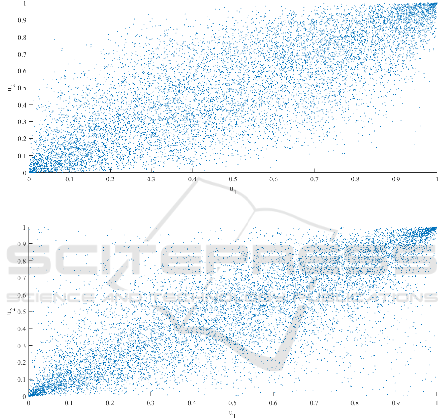
Within the elliptical copulas, t-copula has two

parameters, therefore t-copula offers another feature

more, the tail dependency. Figure 1 shows the scatter

plot of random values generated with a Gaussian

copula, setting the correlation parameter ρ = 0.8, and

with the same correlation parameter and the degrees

of freedom parameter υ = 3, Figure 2 shows the scatter

plot of random values generated with a t-copula.

Visible between these two figures is how the t-

copula can simulate values at the corners of the

distribution space. This flexibility is given by the

parameter degrees of freedom υ. For instance, fixing

the correlation parameter and changing the degrees of

freedom to higher values, in a t-copula density, results

in a Gaussian copula. That said, t-copula is more

flexible than Gaussian and can better fit the data, but

this flexibility results in a costly computation.

Bivariate Gaussian and t-copula are symmetric

copula distributions, but in the Archimedean cases,

only Frank, as shown Figure 3, remain with same

property, Gumbel, and Clayton, shown in Figure 4

and Figure 5, respectively, are not symmetric copulas.

The combination of these five copulas to be used

in the model ensures a wide range of possibilities and

maps the entire distribution space that the data may

Assessing Impacts of Vine-Copula Dependencies: Case Study of a Digital Platform for Overhead Cranes

189

have, as we can see in the scatter plot in the Appendix:

Figures.

Once an overview of copula features has been

described, in the next section we set a copula structure

for assessing the impacts on the Risk Model. Leaving

ready after the discussion, the implementation in

practice with real data.

4 IMPACTS IN THE MODEL

The parameterized scenario as well as the Risk Model

used as the base case for comparison in this

contribution is described in references Szpytko, J. and

Salgado Duarte, Y. (2020b) and Szpytko, J. and

Salgado Duarte, Y. (2021).

In papers cited above, the generation of random

numbers to simulate potential failures in the overhead

cranes were considered independent. Now the

random numbers will be generated using a given

dependency structure.

Figure 5 shows the Risk Model overview and the

convolution product definition to obtain the Loss

Capacity indicator (see references cited for more

details), and in the same diagram, we also point out

the impacted variable by the dependency structure

and its connection with the Risk Model.

The proposed algorithm for generating random

dependent numbers is an independent layer that

transfers the dependencies information to the

simulated vector of potential overhead crane failures.

As a result, the simulation has built-in dependency

information and considers common failure states

between overhead cranes.

In the system analyzed, 33 overhead cranes make

up the system, but only 26 cranes report historical

failures.

Therefore, the vine copula dependency structure

is composed of 25 bivariate copulas concatenated.

For testing purposes, and considering the whole

range of copulas available in our case, we propose to

repeat five times the following five copulas to build

the entire vine copula structure, also following the

order listed below:

- Gaussian copula with parameter ρ = 0.8.

- t-copula with parameter ρ = 0.8 and degrees

of freedom υ = 3.

- Frank, Gumbel, and Clayton copulas, all of

them with parameter θ = 10.

Taking the parametrization of the above described

vine copula and merging the dependency structure

information into the Risk Model adopted, we obtain

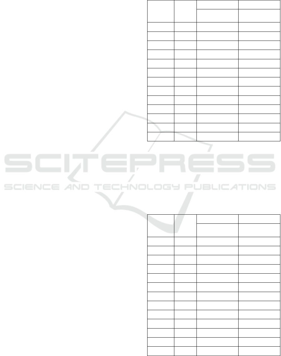
the results in Table 1 and Table 2.

Table 1: Risk value of each scenario evaluated.

Scenario η (%)

Independent Vine copula

Capacity Loss

(

tons/

ear

)

Capacity Loss

(

tons/

ear

)

1 95 19830.88 28191.50

2 94 15809.63 22643.14

3 93 12926.06 18656.09

4 92 10161.75 14868.16

5 91 7730.12 11490.93

6 90 5499.55 8433.81

7 89 3827.58 6146.27

8 88 2717.24 4601.36

9 87 1648.54 3165.55

10 86 1161.59 2297.41

11 85 782.20 1615.97

12 80 111.91 290.17

Base 75 14.61 47.78

Table 1 shows the exponential increasing impact

on the risk indicator assessment when the Risk Model

variables are changed sensitively. The risk indicator

Capacity Loss is the conditional expected value of the

convolution between the available capacity of the

overhead crane system and the number of overhead

cranes required to support the production line.

Table 2: Variance of each scenario evaluated.

Scenario η (%)

Independent Vine copula

Sample

Size

Sample

Size

1 95 202 436

2 94 205 459

3 93 211 470

4 92 224 482

5 91 232 478

6 90 294 569

7 89 384 747

8 88 645 912

9 87 1111 1359

10 86 1214 1424

11 85 1462 1732

12 80 5907 3946

Base 75 28108 14339

EI2N 2021 - IFAC/IFIP International Workshop on Enterprise Integration, Interoperability and Networking

190

Figure 7 shows the visual view of the impact.

When more cranes are required to support the

production line, the risk of Loss Capacity due to

possible unexpected failures increases.

As expected also, when we now consider the

common failures among the overhead cranes, the risk

values per scenario is higher. The reason relates to the

incorporation of the common failure probability

states in the assessment.

In addition, Figure 7 also shows that the impact is

even more severe, in states with a larger convolution

area (see Figure 7 in Appendix, blue line: simulated

independent failures and red line: simulated failures

considering the proposed dependency structure). The

assessment shows a clear impact when considering

common events.

On the other hand, Table 2 shows how the

variance of the estimator behaves. For example, since

the copula approach with the parameters set has a

smaller individual scatter of the random numbers than

the previously generated independent values, as a

result, the system estimator Loss Capacity has less

variance as well.

The results presented in this paper show in some

way the potential impact of considering dependencies

in the adopted model and illustrate the range of

copulas that will be used in future states of research

and applied in practice.

It is important to clarify that in this work, the

figures related to the scatter plots were created using

the same parameterization described at the beginning

of this section.

5 CONCLUSIONS

The algorithm used to evaluate the impact of the

dependency structure on the adopted Risk Model

achieved the expected results. When common failures

between overhead cranes are considered and exist, the

scenario is more severe, and Table 1 and Figure 7 are

the evidence of the conclusion.

The research shows how the vine copula approach

can be applied to historical degradation data, and how

it can be used by the adopted digital platform under

study. This paper leaves the field ready to merge the

dependency measurement with real failure data (vine

copula structure), the risk assessment routines (Model

Risk and the algorithm proposed to simulate

dependent random numbers), and the maintenance

scheduling implemented in the digital platform.

Moreover, it is a clear application of the vine copula

approach.

This methodology can be extrapolated to another

dataset without much effort, following the same idea,

trying to measure certain dependencies between data

vectors corresponding to different components within

the same system.

In future steps of the research, as a continuation of

the presented work, we will share the application of

both stages (measurement and simulation) with real

failure data.

ACKNOWLEDGEMENTS

The work has been financially supported by the

Polish Ministry of Education and Science.

REFERENCES

Aas, K., Czado, C., Frigessi, A., Bakken, H. (2009) Pair-

copula constructions of multiple dependence.

Insurance: Mathematics and Economics. 44 (2009)

182–198.

Bedford, T., Cooke, R. M. (2002). Vines—A New

graphical model for dependent random variables. The

Annals of Statistics. 2002, Vol. 30, No. 4, 1031–1068.

MATLAB. (2019). version 9.7.0.1586710 (R2019b).

Natick, Massachusetts: The MathWorks Inc.

Sun, F., Fu, F., Liao, H., Xu, D. (2020). Analysis of

multivariate dependent accelerated degradation data

using a random-effect general Wiener process and D-

vine Copula. Reliability Engineering and System

Safety. 204 (2020) 107168.

Szpytko, J and Salgado Duarte, Y. (2020). “Integrated

maintenance platform for critical cranes under

operation: Database for maintenance purposes”.

Preprints of the 4th IFAC Workshop on Advanced

Maintenance Engineering, Service and Technology.

September 10-11, 2020. Cambridge, UK.

Szpytko, J. and Salgado Duarte, Y. (2020). “Exploitation

Efficiency System of Crane based on Risk

Management”. Proceedings of International

Conference on Innovative Intelligent Industrial

Production and Logistics, IN4PL 2020. 2-4 November

2020.

Szpytko, J. and Salgado Duarte, Y. (2021). Technical

Devices Degradation Self-Analysis for Self-

Maintenance Strategy: Crane Case Study. Proceedings

of INCOM 2021, June 2021, 17th IFAC Symposium on

Information Control Problems in Manufacturing.

Szpytko, J. and Salgado Duarte, Y. (2022). Digital Platform

for Overhead Cranes Maintenance Strategies:

Measuring Dependencies on Degradation Data with Vine

Copulas. Manuscript submitted to 14th IFAC

Workshop on Intelligent Manufacturing Systems.

Received July 20, 2021.

Assessing Impacts of Vine-Copula Dependencies: Case Study of a Digital Platform for Overhead Cranes

191

APPENDIX

Figures

Figure 1: Scatter plot of a Gaussian copula.

Figure 2: Scatter plot of a t copula.

EI2N 2021 - IFAC/IFIP International Workshop on Enterprise Integration, Interoperability and Networking

192

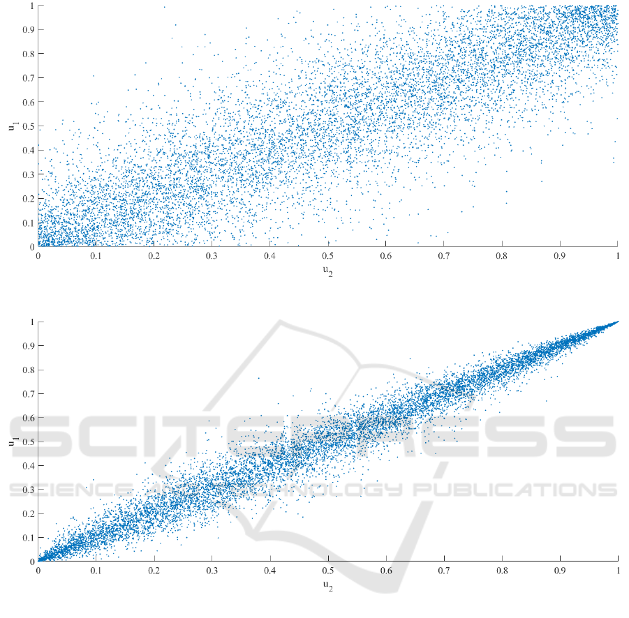
Figure 3: Scatter plot of a Frank copula.

Figure 4: Scatter plot of a Gumbel copula.

Assessing Impacts of Vine-Copula Dependencies: Case Study of a Digital Platform for Overhead Cranes

193

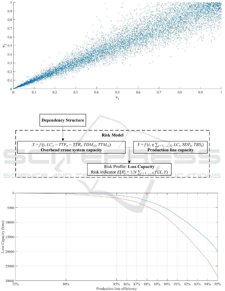
Figure 5: Scatter plot of a Clayton copula.

Figure 6: Risk Model architecture.

Figure 7: Dependency structure impact on the model.

EI2N 2021 - IFAC/IFIP International Workshop on Enterprise Integration, Interoperability and Networking

194

Generating Random Numbers with Vine Copula:

1.- For sampling ~u dependent uniform random

numbers [0, 1] with a vine copula, defining ~u

d,n

as a

d × n matrix, where d is the dimension and n is the

length of the random sample, first we need an w

independent uniform random sample [0, 1] as starting

point, then with the vine copula concatenation

estimated, we apply the following steps by u

component considered:

()

221

3312

ddd

uFuu

uFuuu

uFuu u

−





where w is a settled random number sample with

length n, and

()F

−

⋅ is a cumulative bivariate copula

density.

In this research, we consider five copula densities

(see Appendix: Bivariate copula densities), therefore,

()F

−

⋅ depends on the k-th bivariate copula density

used. Below we describe the steps performed

depending on the copula used, where v

and v

variables represent the pair correlated vector in each

step and w independent uniform random sample or a

sample vector of the previous concatenation step:

a.- If k-th copula density is Clayton: v

= w,

then

21 1

1vvp v

−









=−+





where θ is the copula

parameter defined 0 < θ < ∞ and p is an independent

uniform random sample [0, 1].

b.- If k-th copula density is Frank: v

= w, then

−





−









=−



−





where θ is the copula

parameter defined -∞ < θ < ∞ and p is an independent

uniform random sample [0, 1].

c.- If k-th copula density is Gumbel: v

= w –

5π, then by successive transformation we obtain:

= v

+ π /2,

ep=−

where p is an independent

uniform random sample, d = 1 and n = sample size,

cos



−





where θ is the copula

parameter defined 1 ≤ θ < ∞ and,

()

sin

cos











=−

where p is an independent

uniform random sample, d = 2 and n = sample size,

−

= v

d = 2,n

d.- If k-th copula density is t: first, given ρ

parameter, a positive correlation matrix, apply the T

Cholesky-like decomposition for covariance matrix,

such as ρ = T

T, and set v

= z (w), where z ( ) is a

normalization function, which centers the data to

have mean equal to 0 and scales it to have standard

deviation equal to 1. Then by successive

transformations:

r = v

1, n

, p

1, n

where p is an independent random

sample,

r = r × T,









where η is the degrees of

freedom, Γ() is the gamma distribution, d = 2 and n

sample size.

r = r / x,

v = t (r, η) where t ( ) is the cumulative t

distribution, then v

= v

d = 1, n

e.- If k-th copula density is Gaussian: first,

given ρ parameter, a positive correlation matrix,

apply the T Cholesky-like decomposition for

covariance matrix, such as ρ = T

T, and set v

= z (w),

where z ( ) is a normalization function, which centers

the data to have mean equal to 0 and scales it to have

standard deviation equal to 1. Then by successive

transformations:

r = v

1, n

, p

1, n

where p is an independent random

sample,

r = r × T,

v = Normal (r) where Normal ( ) is the

cumulative Gaussian distribution, then v

= v

d = 1, n

2.- End of sampling ~u dependent uniform random

numbers [0, 1] with a vine copula. As a result, a

matrix of uniform dependent random numbers is

obtained.

Bivariate Copula Densities:

In this document we present five possible selections

in the bivariate copula fitting process performed for

continuous variables. Below we describe the list of

Assessing Impacts of Vine-Copula Dependencies: Case Study of a Digital Platform for Overhead Cranes

195

probability copula density functions used in the

selection.

1.- Clayton:

()

12 1 2

,; 1cu u u u

θθ

−

−−

=+−

where θ

is the copula parameter defined 0 < θ < ∞.

2.- Frank:

()

()()

ln 1 1

cu u

θθ

−−

−

−−−

−

where θ is the copula parameter defined -∞ < θ < ∞.

3.- Gumbel:

()

()( )

ln ln

cu u e

θθ



−− +−





where θ

is the copula parameter defined 1 ≤ θ < ∞.

4.- Gaussian:

() ()()

12 1 2

,; ,cu u u u

−−



=Φ Φ Φ



where ρ is a pairwise correlation value defined -1 < ρ

< 1.

5.- t-copula:

()()()

12 , 1 2

,;, ,cuu t tutu

υρ υ υ

υρ

−−





where ρ is a pairwise correlation value defined -1 < ρ

< 1 and υ is the degrees of freedom parameter defined

υ > 1.

EI2N 2021 - IFAC/IFIP International Workshop on Enterprise Integration, Interoperability and Networking

196