Honeycomb Layout Inspired Motion of Robots for Topological Mapping

Raul F. Santana and George A. P. Th

Department of Teleinformatics, Federal University of Cear

a, Fortaleza, Cear

a, Brazil

Keywords:

Robot Swarm, Collaborative Robotics, Mapping, Topological Maps.

Abstract:

Swarm robots are an important area of mobile robotics inspired by the collective behavior of animals for the

execution of activities and, using this premise, the present work aims to present a swarm robotics algorithm

for topological mapping of environments. A comparison was made with another article in the literature that

presents a similar technique, where it was possible to see an improvement in performance in the proposed

parameters. An assessment of closed-loop control was also carried out, using a proposed evaluation metric,

which showed a minor impact with the increase in the number of agents, and in smaller environments.

1 INTRODUCTION

Bioinspired motion of robots swarm aimed at repro-

ducing the behaviour of birds, ﬁsh, bees etc has re-

ceived intensive attention lately (Barca and Seker-

cioglu, 2013). The ability to cooperate in coordinated

group tasks opens up a wide range of interesting ap-

plications in the ﬁeld of logistics (Wen et al., 2018)

and environment exploration (Ramachandran et al.,

2017). Indeed, one of the most basic issue in robotics,

navigation is especially important in unknown scenar-

ios, since it allows for gathering environment infor-

mation in the fundamental task called mapping, as in

SLAM applications (Choset et al., 2005).

Mapping consists of creating spatial models for

the environment from sensor perception and can be

divided into three main categories: geometric, topo-

logical and grid maps. In geometric maps, there are

primitive geometric shapes which rely on parameter

adjustment able to suitably ﬁt the information com-

ing from the sensors. Grid maps, in turn, rely on spa-

tial grid representation for a scene, with an occupancy

probability being associated to the cells; it is a not

scalable alternative, and leads to problems in case of

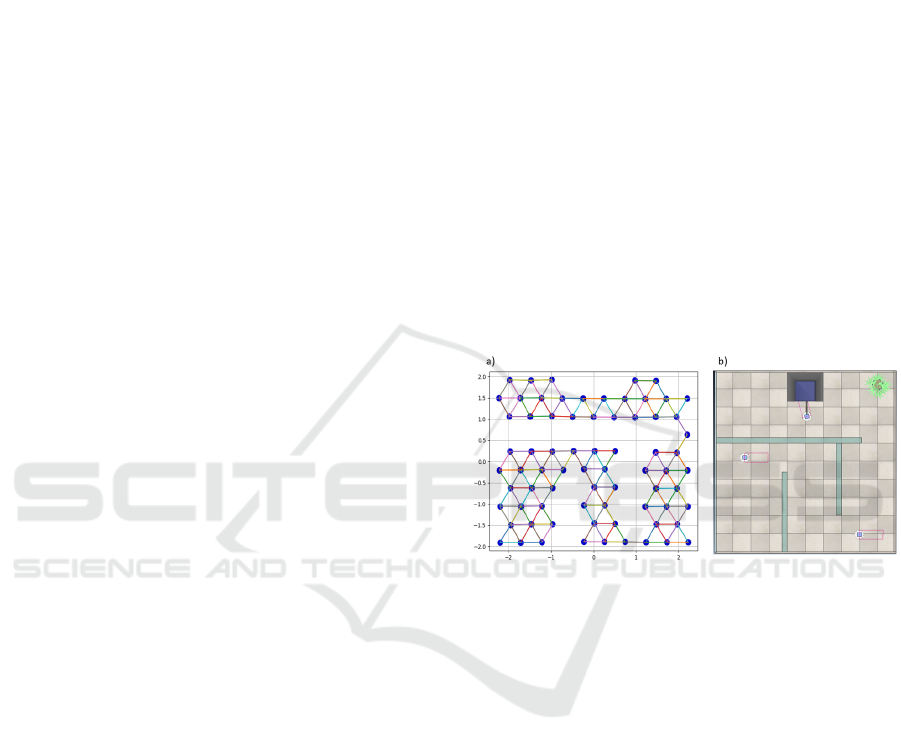
large environments. Finally, topological maps repre-

sent the environment in the form of nodes and edges

for the free-collision regions, as in Figure 1a, where

each node represents a place of interest, and the edges,

their connections (Akdeniz and Bozma, 2015).

In the literature, a huge amount of works report

on the use of robot swarms in the task of topologi-

cal mapping (Akdeniz and Bozma, 2015; Dirafzoon

et al., 2017). For instance, drones were used in aerial

mapping after earthquakes (da Rosa et al., 2020),

Figure 1: Example of topological map and work issues.

swarms of wheeled-robots mapped industrial ware-

houses (Marjovi et al., 2010) and intelligent vacuum

cleaners were engineered to collectively search for ol-

factory sources in a industrial shed (Marjovi and Mar-

ques, 2011).

In this context, here the topological mapping of

typical indoor scenarios, as the one illustrated in Fig-

ure 1b is addressed from a honeycomb geometry

inspired algorithm for the motion-level decision of

wheeled robots. In the investigation, issues like the

environment size and the existence of position closed-

loop control are discussed and an error metrics for the

quality of the produced maps is proposed.

2 THEORETICAL BACKGROUND

2.1 Depth-ﬁrst Search

The Depth-First Search algorithm is a routine for ex-

ploring graphs in the form of trees, often used to

Santana, R. and Thé, G.

Honeycomb Layout Inspired Motion of Robots for Topological Mapping.

DOI: 10.5220/0010709600003061

In Proceedings of the 2nd International Conference on Robotics, Computer Vision and Intelligent Systems (ROBOVIS 2021), pages 143-149

ISBN: 978-989-758-537-1

143

search for elements within the tree. The algorithm

starts with choosing an arbitrary node to be the root of

the tree and from it new descending nodes are added

to complete the tree (Skiena, 2020).

The process of adding nodes consists of going

from ancestral nodes to descendants until all descen-

dants have been explored. Once a descendant is cho-

sen to start the exploration, the process of choosing

a new child will be recursive until the last child node

has no more children. Once reached the end of the

branch, the algorithm will return to the closest ances-

tor that still has unexplored children and will choose a

new node to be explored, restarting the cycle. In order

to avoid inﬁnite cycles, each node should be explored

only once, which implies not revisiting an already ex-

plored node, even if it is accessible from another an-

cestral node. The routine comes to an end when there

are no more nodes to explore (Skiena, 2020).

Edges connecting nodes are classiﬁed into two

categories in non-directional graphs: tree edges and

back edges. While the edges of the tree link nodes

from ancestor to descendants, the backlinks descen-

dants to ancestors, guaranteeing a return to parent

nodes, so that exploration of other descendants is al-

lowed (Skiena, 2020).

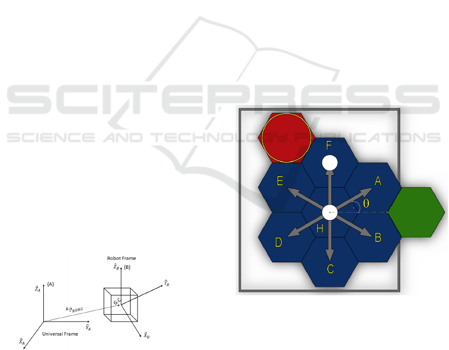
2.2 Spatial Representation

For what concerns the spatial representation in the

navigation simulations reported hereafter, it is to be

mentioned that all the scenarios are in-plane motion

and, as such, a simple description for position and ori-

entation is considered. The approach here adopted is

according to (Craig, 2009), in which the position of a

mobile robot in the scene is given by the vector locat-

ing the origin of frame B respect to the universal coor-

dinate system A, whereas the robot orientation may be

retrieved from the rotation matrix calculated from the

inner-product between unit-vectors of principal axes

relating frames B and A.

Figure 2: Relative frame description of universal and local

coordinate systems.

3 METHODOLOGY

This section presents in detail the implemented algo-

rithm for topological mapping. It is based on the con-

tribution brought by others in (da Rosa et al., 2020)

in that, the hexagon-like layout of the scene was im-

plemented accordingly, but some improvements have

been made in the motion rules, in the perception of

the neighborhood, in the path planning and movement

control, so that maps are generated more accurately

and efﬁciently.

n the hexagon-like layout for the scene, robot

scans move in the orthogonal direction to the hexagon

faces, thus limiting motion orientation to the set

,90

, 150

, 210

, 270

, and 330

, as shown in Fig-

ure 3. A free node is deﬁned as the hexagon center

when it is empty (no robots occupying) or accessible

without collision (think of other objects in the scene).

In the picture, cells A, B, C, D, E, and F are neighbors

nodes and are accessible from the current position of

the agent (white circle in H cell); the red node is not

in the agent’s neighborhood, being accessible only by

nodes E and F, and the green hexagon is not part of

the map, since its center lies outside the room. It is

a premise that each element of the swarm has access

to its global position and can communicate with other

agents at any time.

Figure 3: Structure of accessible and non-accessible neigh-

boring nodes.

Figure 4 shows the ﬂowchart of the algorithm

used, which is inspired by the depth-ﬁrst search tech-

nique presented in subsection 2.1, where a branch

must be explored until there are no more unvisited

descendants before exploring a new branch. To do

this, robots share a list of explored nodes and one of

the unexplored nodes, and as a new node is visited, it

ROBOVIS 2021 - 2nd International Conference on Robotics, Computer Vision and Intelligent Systems

144

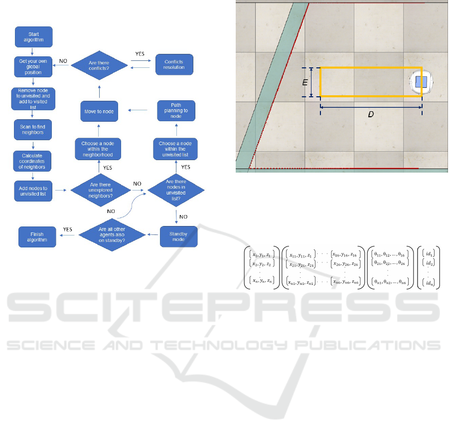
gets inserted into the list of visited nodes and removed

from the list of unvisited nodes.

Figure 4: Flowchart of the mapping algorithm embedded in

robots.

An important equipment in the mapping is the Li-

DAR sensor; indeed, by using it to circularly scan the

environment, new nodes (both neighbors or descen-

dants) can be discovered. Every time a free node is

found and hence available to be visited, its coordi-

nates are computed in a universal frame and inserted

into the list of unvisited nodes and added to the part of

the neighborhood of the current node data struct. Its

orientation comes along. The main reason for choos-

ing the LiDAR sensor was its zone-sensing perception

ability which allows creating, using basic geometric

calculations, a clear safe zone for prompt collision

avoidance. Figure 5 shows the safe zone mentioned in

yellow, while D represents the distance to be moved

and E gives the robot’s diameter. It should be stressed

that these details about the neighborhood perception

and on the choice of LiDAR for safe zone purposes

are missed in the literature.

The map itself is a data structure, as shown Figure

in 6, cointaining the node coordinates, its neighbors,

as well as the orientation and an identiﬁcation of the

agent that visited the node. At the end of the scan

process, the current node is added to the map. After

that, the robot chooses the next destination to visit,

and will do this into unvisited list, giving preference

to node in it neighborhood. If there no unvisited node

in neighborhood, the robot has two rules to choose:

First In First Out (FIFO) and Euclidian distance. In

the ﬁrst one, the robot will choose the ﬁrst node added

Figure 5: Use of the LIDAR sensor and the projected safety

zone.

in unvisited list, while in the second rule, the robot

will choose the node with shorter Euclidian distance

for the current node.

Figure 6: Structure of the map used.

Differently to (da Rosa et al., 2020), in the present

work, the decision rule for motion always favors the

neighbor nodes. Another difference regards the dis-

tance metric which is here dependent on the initial

node position, and not on the robot’s current position

as in (da Rosa et al., 2020).

Once the next objective is clear, a route is de-

ﬁned according to the A* path-planning algorithm,

and the navigation among nodes follows similarly to

what happened in the case of descendant nodes. Such

a repeated process of recalculating movement param-

eters, even in known areas, aims at mitigating the

propagation of position error. As the current map

uses a global coordinates approach, it is more sus-

ceptible to error accumulation than probabilistic ap-

proaches such as (Dirafzoon and Lobaton, 2013; Di-

rafzoon et al., 2014; Dirafzoon et al., 2017). To

cope with that, a PID-controller was implemented for

set-point control at the orientation-level. Parameters

tuning followed Ziegler-Nichols approach, and led to

= 0.28, K

= 0.008 and K

= 0.0009.

3.1 Collision Prevention

An important issue in robot navigation, collision

avoidance plays a fundamental role in map generation

from groups of agents. The good news is that the dis-

Honeycomb Layout Inspired Motion of Robots for Topological Mapping

145

cretized nature of the spatial representation allows for

the use of simple rules for preventing multiple node

occupancy and for preventing agents to assume close

goal positions. In the environment exploration, goal

scan be categorized into two types: next objective and

ﬁnal objective. The ﬁrst one concerns the adjacent

nodes, whereas the latter is related to a distant cell to

be reached.

A good strategy for collision avoidance required

the agents to have access to others’ objectives in such

a way to properly check in the list of unvisited nodes

about the intention of other agents. A typical collision

situation may occur in a movement to a distant ﬁnal

objective; in this case, the waypoints can be in the

en-route path of other agents and, to properly prevent

the collision, preference is given to the agent that ﬁrst

published that node as a next objective.

3.2 Conﬂict Resolution and Exploration

Completion

The above-mentioned conﬂict of interests of differ-

ent agents to visit simultaneously a given node is es-

pecially frequent in small-size environments. A way

to deal with that is to deﬁne different states for the

agents and to share this information with every other

robot in the task. In the present work, a number of 4

(four) activity modes were deﬁned: standby, explor-

ing, moving, and conﬂict. Once there is active conﬂict

detected, the agent is put on standby giving free pas-

sage to the agent which preceded the motion. In the

case the path remains blocked, the agent undergoes

the conﬂict mode, and passing priority is assigned to

the robot with more free neighbors in its vicinity; the

others, which are in conﬂict, must wait. This can be

illustrated with the help of Figure 3, in which nodes

A and E are blocked, and the robot occupying node

Hmust leave its location, since it has free neighbors

B, C, and D. At the end of that node access negoti-

ation, the objectives must be recalculated and, if the

conﬂict persists, the process goes to new rounds until

no conﬂict is left.

The standby mode is also assumed when the ex-

ploration is completed (meaning that no nodes in the

unvisited list are left). In this case, the robots wait

collectively for the activation of standby mode of ev-

ery other in the group. Only in that condition, the

algorithm reaches completion. Finally, to be stressed

that a robot enters standby mode does not prevent new

conﬂicts to arise; hence, the standby mode does not

exempt the robot to act to solve them by giving a free

pass to other agents.

4 RESULTS

Aiming at bringing new contributions to the state of

the art, in this section, the discussion focuses on the

quality of the map, an issue that has been neglected

in the recent literature. The study comprehends sim-

ulations done in CoppeliaSim Software, which is an

integrated development environment for simulations

of factory automation systems and robotics based on

a distributed control architecture. It supports devel-

opment through application interfaces for many pro-

gramming languages including Python, which was

used in the present work. A number of up to 3 (three)

Khepera III model robots were used, equipped with

the LiDAR sensor, which covered an area of nearly

100 m

deﬁned by 0.5 meters-spaced hexagon-like

cells, with Euclidean distance based exploration rule.

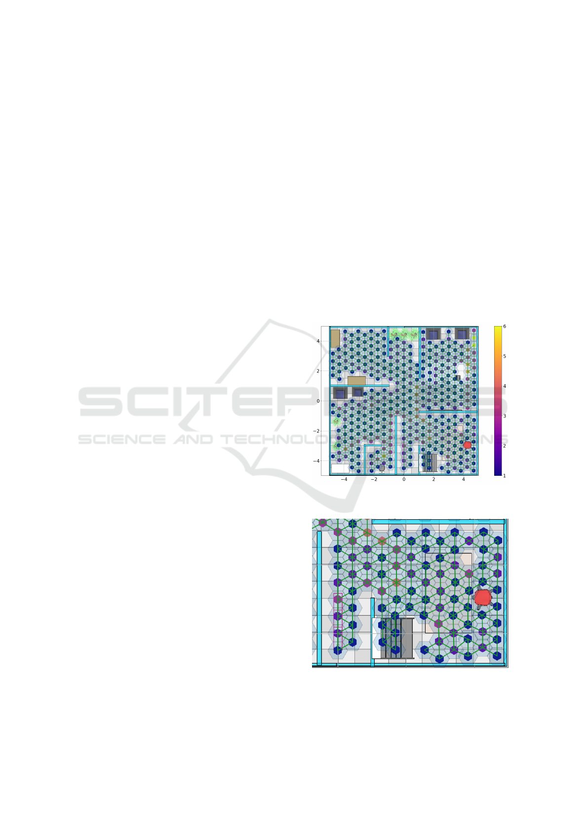
4.1 Preliminar Evaluation

Figure 7: Modeled scenario for validation of the algorithm

and its respective map.

Figure 8: Zoom view of the modeled scenario, with its re-

spective map.

ROBOVIS 2021 - 2nd International Conference on Robotics, Computer Vision and Intelligent Systems

146

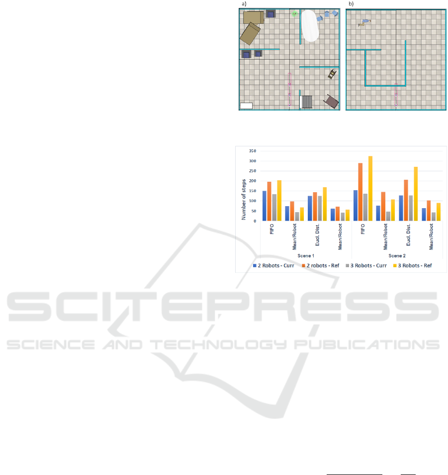
Figure 7 shows the ﬁrst modeled environment and

its respective map, with the color information repre-

senting the visitation frequency as a heat map accord-

ing to the scale shown in the right side. The pic-

ture shows very good coverage of the environment.

In its expanded view, in Figure 7, it is possible to

see no overlap between obstacles and centers of cells;

in addition, there are no edges connecting neighbor-

ing nodes with obstacles between them, which may

indicate an absence of collision with them. On the

other hand, the map brings small overlaps between the

hexagons, which implies that we have different posi-

tions from those initially idealized, a fact that moti-

vated the upcoming discussion of movement control.

4.2 Comparison with the Literature

To provide a fair comparison to paper (da Rosa et al.,

2020), this part of the study relies on the the amount

of steps needed to carry out the mapping as a met-

ric. Also, preference is given to scenes already inves-

tigated in that paper, which were carefully reproduced

in every detail and are reported in Figure 9.

The bar-graph in Figure 10 presents the results ob-

tained with two and three robots in both scenarios (la-

bel Ref means the literature paper used for benchmark

(da Rosa et al., 2020)). It is possible to notice in the

results of the present work a pattern of reduction of

the number of steps with the increase of the number of

robots, for both scenarios in the FIFO conﬁguration,

constraining the stabilization of the same parameter in

the Euclidean distance conﬁguration. The pattern of

reducing the average number of steps per robot with

increasing them was maintained in both works. The

reference work presented variations for the FIFO and

Euclidean Distance settings of 31.63% and 21.21%,

respectively, for scenario 1, and 25.51% and 12.29%

for the other, while the present work presented vari-

ations of 40%, 33.33%, 40.37% and 33.33% for the

same cases, which represents a greater impact of the

number of robots on the number of steps in the present

algorithm. Also to be mentioned is the absolute num-

ber of steps indicating better efﬁciency on robots’

motion during the mapping produced by the present

work.

4.3 Evaluation Metrics

A gap found in the reference literature concerns the

evaluation of the quality of the generated topological

map, so one of the contributions of this work is the

introduction of an error metric that allows evaluating

which factors inﬂuence the quality of the map built.

It is an adimensional number relying on two terms:

Figure 9: Modeled scenarios for comparison, as introduced

by (da Rosa et al., 2020).

Figure 10: Comparison between models. Label ”Curr”

means this work.

one for the distance between neighboring nodes and

the other, for the angle between them, according to

equation 1. It accounts for the difference between

the threshold, representing the idealized distance be-

tween neighboring nodes, and the actual distance be-

tween the same. Same rationale applies for the orien-

tation. A weighting factor is also considered to allow

for tuning of both aspects (position and orientation);

this way, β = 0 leads to a positioning error metrics,

whereas β = 1 leads to an orientation error metrics.

Anything in between gives a general error metrics en-

compassing both of them and, as such, may be seen

as a ﬁgure-of-merit.

error =

∑

((1 − β)

∆Distance

thresholdDist

+ β

∆θ

180

) (1)

4.4 Movement Control Evaluation

As the reader should be aware of, positioning is an

essential task for obtaining good mapping. It is there-

fore important for the robots to have a good position

closed-loop control at the motion level. In this sec-

tion we investigate how the mapping performs with

and without closed-loop control at the motion level.

The investigation also includes the role of the environ-

ment size (from 4 up to 10 meters-side square rooms)

Honeycomb Layout Inspired Motion of Robots for Topological Mapping

147

and the role of amount of agents. The rule for non-

neighbor nodes is based on Euclidean distance with

0.5m separation between cells.

With β = 0.5, Figure 11 brings at a glance a num-

ber of important trends. Firstly, the importance of

closed-loop control; can positively affect the quality

of the maps as measured by the formerly introduced

error metrics. Secondly, it is clear that the larger the

area to cover, the worse the map generated, which

might be speculated to be associated with the need

to compute more displacements among cells in large

environments. This is, however, compensated by the

inclusion of more robots in the task, as it can be seen

in the picture as the amount of robots goes from one

to three. The third conclusion, indeed, somehow sug-

gests that the decrease in the average amount of steps

favors the speculation above. With no great ambi-

tions, we could synthesize the idea of ”the less you

walk, the better the map gets”, thus pointing to the

real beneﬁt of a group and coordinated activity of mo-

bile agents.

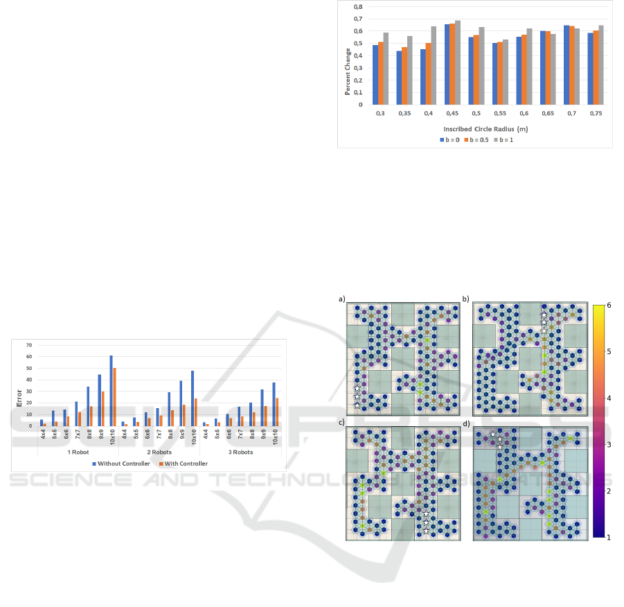
Figure 11: Error metrics by environment and by number of

robots.

Moving on, we put light to the map resolution.

To see the the role of the closed-loop control, map-

ping was carried out in a 49 m

square-like environ-

ment having three mobile agents, and the size of the

hexagon-cells were modiﬁed. The hexagon-inscribed

circle’ diameter ranged from 0.3 to 0.75 meters in this

experiment.

The percentage variation of the error was inves-

tigated in this map-resolution study. Results are

brought in Figure 12, for different values of β. Here,

percentage is calculated as the relation between the

error deviation with-without controller and the error

without controler.

Analyzing the graph, it is possible to see that, for

the most part, the percentage variation of the error is

greater for β = 1, which means a greater difference

between the error related to direction between a plant

that uses and one that does not use a controller, show-

ing that the controller has greater ability to mitigate

this type of error.

Figure 12: Error variation between situations with and with-

out controller, for different offset distances.

We conclude that the presence of a controller is

essential once again to limit the error and provide a

good mapping.

4.5 Inﬂuence of Starting Position

Figure 13: Maps generated by robots with changing starting

positions.

To see if and how the robots’ initial position could

affect the map, we assessed the heat map for a given

scene from 3 different initial positions. In Figure 13,

these are indicated with white stars. From each gener-

ated map, in terms of completeness of the swept area,

no relevant differences were observed. It is to be men-

tioned, however, a certain inﬂuence of the agents’ ini-

tial position on the incidence of the heat map, where

the nodes of the maps 13c and d had greater trafﬁc on

the left side in comparison to the others. In addition,

it can be observed a higher number of steps per node,

which suggests a correlation between the distribution

of agents on the map with the initial conditions of the

scene, especially in the vicinity of the agents.

ROBOVIS 2021 - 2nd International Conference on Robotics, Computer Vision and Intelligent Systems

148

5 CONCLUSIONS

In the present work, a robot swarm algorithm for ex-

ploration and topological mapping of environments

was introduced and compared to a recent contribution

of the literature. The study carried out focused on the

quality of the generated maps as measured by a sim-

ple ﬁgure-of-merit metric here introduced. It was also

investigated the role of the number of agents, the chal-

lenges posed by the environment size, and the effects

on the close-loop control strategy for robot position-

ing. The analysis revealed that the present implemen-

tation was very efﬁcient in terms of computation steps

when building the maps, which points to a good per-

spective regarding the power consumption of robots.

The discussion on motion close-loop control showed

the importance of relying on it for efﬁcient map gen-

eration and, associated with that, revealed that it ben-

eﬁts hugely as the population of agents grows.

As future work, we suggest the investigation of

new business decision rules for accessing nodes to

visit, to maximize agents’ parallelism, thus reducing

the visitation rates of nodes and maximizing robots

exploration performance.

REFERENCES

Akdeniz, B. C. and Bozma, H. I. (2015). Exploration and

topological map building in unknown environments.

In 2015 IEEE International Conference on Robotics

and Automation (ICRA), pages 1079–1084. IEEE.

Barca, J. C. and Sekercioglu, Y. A. (2013). Swarm robotics

reviewed. Robotica, 31(3):345–359.

Choset, H. M., Hutchinson, S., Lynch, K. M., Kantor, G.,

Burgard, W., Kavraki, L. E., and Thrun, S. (2005).

Principles of robot motion: theory, algorithms, and

implementation. MIT press.

Craig, J. J. (2009). Introduction to robotics: mechanics and

control, 3/E. Pearson Education India.

da Rosa, R., Aurelio Wehrmeister, M., Brito, T., Lima, J. L.,

and Pereira, A. I. P. N. (2020). Honeycomb map: a

bioinspired topological map for indoor search and res-

cue unmanned aerial vehicles. Sensors, 20(3):907.

Dirafzoon, A., Betthauser, J., Schornick, J., Benavides, D.,

and Lobaton, E. (2014). Mapping of unknown en-

vironments using minimal sensing from a stochastic

swarm. In 2014 IEEE/RSJ International Conference

on Intelligent Robots and Systems, pages 3842–3849.

IEEE.

Dirafzoon, A., Bozkurt, A., and Lobaton, E. (2017). A

framework for mapping with biobotic insect networks:

From local to global maps. Robotics and Autonomous

Systems, 88:79–96.

Dirafzoon, A. and Lobaton, E. (2013). Topological map-

ping of unknown environments using an unlocal-

ized robotic swarm. In 2013 IEEE/RSJ International

Conference on Intelligent Robots and Systems, pages

5545–5551. IEEE.

Marjovi, A. and Marques, L. (2011). Multi-robot olfactory

search in structured environments. Robotics and Au-

tonomous Systems, 59(11):867–881.

Marjovi, A., Nunes, J. G., Marques, L., and de Almeida, A.

(2010). Multi-robot ﬁre searching in unknown envi-

ronment. In Field and Service Robotics, pages 341–

351. Springer.

Ramachandran, R. K., Wilson, S., and Berman, S. (2017).

A probabilistic approach to automated construction of

topological maps using a stochastic robotic swarm.

IEEE Robotics and Automation Letters, 2(2):616–623.

Skiena, S. S. (2020). The algorithm design manual.

Springer International Publishing.

Wen, J., He, L., and Zhu, F. (2018). Swarm robotics con-

trol and communications: imminent challenges for

next generation smart logistics. IEEE Communica-

tions Magazine, 56(7):102–107.

Honeycomb Layout Inspired Motion of Robots for Topological Mapping

149