Per-flow Packet Loss Ratios Induced by an Overflowed Buffer
Andrzej Chydzinski
a
and Blazej Adamczyk
b
Silesian University of Technology, Department of Computer Networks and Systems, Gliwice, Poland
Keywords:
Buffer Overflow, Packet Loss, Loss Ratio, Per-flow Analysis.
Abstract:
Packet losses are common in TCP/IP networks. The main reason of that is the statistical multiplexing of flows
at routers’ output buffers, resulting in random overflows of these buffers and dropping of packets. Although
the losses caused by an overflowed buffer have been widely studied, these studies were mainly devoted to the
aggregated traffic. Namely, the total loss ratio was analyzed, for all the packets arriving to the buffer, without
distinction between separate flows. In this paper, we study the packet loss ratios suffered by distinct flows
arriving to a common buffer. We first observe that the loss ratios of particular flows may differ significantly
from each other, and from the total loss ratio. Then we single out the properties of the flow that may influence
the per-flow loss ratio. We study also possible mutual dependencies between the flows, i.e. possibilities that
the properties of one flow influence the loss ratios of other flows. Finally, we study the impact of the buffer
size and the distribution of the service time (packet size) on the per-flow loss ratios, as well as their relations
to ech other.
1 INTRODUCTION
In an IP router, all the flows bound to a particular
output interface have to share a common buffer. As
the packets from all these flows are statistically multi-
plexed upon arrival to this buffer, some random bursts
may occur, overflowing the buffer and making it tem-
porarily unavailable. Other packets, arriving to the
buffer during such overflow periods, are deleted and
lost.
As long as the network operates in the ”best ef-
fort” manner, without allocation of resources, such
losses are unavoidable. In fact, they are common in
most TCP/IP networks and the Internet.
The main characteristic of the loss process is the
loss ratio, L, defined as the number of lost packets di-
vided by the total number of packets, in a long time
interval. This characteristic has been widely stud-
ied using mathematical models (Takagi, 1993; Yajnik
et al., 1999; Sanneck and Carle, 1999; Yu et al., 2005;
Hasslinger and Hohlfeld, 2008; Chydzinski et al.,
2007; Chydzinski and Adamczyk, 2012) and net-
work measurements (Bolot, 1993; Coates and Nowak,
2000; Benko and Veres, 2002; Duffield et al., 2001;
Sommers et al., 2005). The loss process has been
also studied with regards to its statistical structure,
a
https://orcid.org/0000-0002-0168-6919
b
https://orcid.org/0000-0001-5038-6309
i.e. the occurrence of losses in groups, one after an-
other (Cidon et al., 1993; Bratiychuk and Chydzinski,
2009). Especially useful in such studies is the packet
burst ratio parameter (McGowan, 2005), which ex-
presses directly the tendency of losses to group to-
gether, in long series. The packet burst ratio has been
analyzed via mathematical models (Rachwalski and
Papir, 2014; Rachwalski and Papir, 2015; Chydzin-
ski et al., 2018; Chydzinski and Samociuk, 2019) and
actual network measurements (Samociuk et al., 2018;
Samociuk and Barczyk, 2019).
Naturally, packet losses can be studied globally (in
the whole network), or in the end-to-end manner, or at
the particular output interface of a networking device.
In this paper we deal with the latter case, i.e. we study
the loss ratio caused by a single overflowed buffer, in
which many flows are statistically multiplexed.
The previous studies of the loss ratio induced by
an overflow buffer lack the distinction between the
loss ratios experienced by particular flows traversing
the common output interface. It is not clear, whether
all the flows sharing a common buffer suffer from the
overflow events in the same way. In other words, it
is not clear, if their private loss ratios are the same as
the total loss ratio, counted for the aggregate traffic.
Or, maybe the loss ratio of an individual flow can be
much higher, or lower, than the total loss ratio, de-
pending on the properties of that flow?
Chydzinski, A. and Adamczyk, B.
Per-flow Packet Loss Ratios Induced by an Overflowed Buffer.
DOI: 10.5220/0010708500003058
In Proceedings of the 17th International Conference on Web Information Systems and Technologies (WEBIST 2021), pages 621-628
ISBN: 978-989-758-536-4; ISSN: 2184-3252
Copyright
c
 2021 by SCITEPRESS – Science and Technology Publications, Lda. All rights reserved
621

In this paper, we show firstly that the latter is true.
Indeed, the per-flow loss ratios may differ signifi-
cantly from each other, and from the total loss ratio,
depending on the statistical properties of flows. Sur-
prisingly, this can happen even if the arrival rates of
all the flows are exactly the same, or even if the inter-
arrival time distributions of all flows are of the same
type.
Secondly, we show the influence of the standard
deviation of the interarrival time of a flow on its pri-
vate loss ratio. As we will see, the per-flow loss ratio,
and the total loss ratio, grow with the standard devia-
tion of the considered flow. What is more surprising,
is that the loss ratios of other flows may stay virtually
unaltered, even if the total loss ratio and the ratio of
one flow change by an order of magnitude.
Thirdly, we study the impact of the buffer size and
the distribution of the service time (packet size) on
the per-flow loss ratios. It is known that the total loss
ratio grows with the standard deviation of the packet
size, and shrinks with the buffer size. It will be shown
that the same is true for the per-flow loss ratios. More
interesting, however, is the relation between the per-
flow loss ratios, when the standard deviation of the
packet size and the buffer size change. For instance,
imagine we have 2 flows with the per-flow loss ratios
of L
1
= 1% and L
2
= 3%. Therefore, we have the
following proportion:
L
2
L
1
= 3. Will this proportion be
kept, if we double the buffer size? Will it be kept, if
we double the standard deviation of the packet size?
As we will see, one of these answers is positive, while
the other is negative.
The per-flow loss ratios are, obviously, of great
importance in the QoS context. Namely, each individ-
ual flow may transport the content of a different type,
e.g. data, audio, video. If the per flow-loss ratios dif-
fer between flows, and the differences depend on the
statistical properties of flows, then we may expect dif-
ferent QoS parameters for data, audio and video flows
sharing the same output buffer.
Unfortunately, there are no mathematical theo-
rems on the per-flow loss ratios in queueing models
with a single buffer and multiple flows arriving to it.
The known formulas concern only the total loss ratio,
for the aggregated traffic (some of them will be re-
called in Section 3). Therefore, a discrete-event sim-
ulator Omnet++ is used for computing the per-flow
loss ratios in this study. Due to the high efficiency of
the simulator, programmed directly in C++ language,
it is possible to simulate, in a rather short time, tens
of millions of packets passing through the buffer. This
is more than enough for the purpose of the loss ratio
analysis carried out in this paper.
The rest of the paper is organized in the following
manner. In Section 2, the queueing model of a buffer
serving multiple flows is formally defined. In Section
3, some known formulas on the aggregated loss ratio
are recalled. In Section 4, the simulation results are
presented and discussed. In particular, nine different
scenarios with different flow types, service time dis-
tributions and buffer sizes are considered. The final
conclusions are gathered in Section 5, and accompa-
nied by some future work suggestions.
2 THE MODEL
Figure 1: The model of the queue.
The scheme of the queueing model analyzed herein is
depicted in Fig. 1. Namely, there are N flows arriving
to a common buffer of size b packets (including the
service position). The packets from all the flows are
placed serially in the buffer, in the arrival order.
Each flow has a form of a separate renewal pro-
cess. Namely, within the i-th flow, all the packet in-
terarrival times are identically distributed, with dis-
tribution function G
i
. Different flows, however, may
have different interarrival time distributions. Thus in
general it can be G
i
6= G
j
.
The buffer is served in the usual FIFO discipline.
The service time of a packet has some distribution
given by distribution function F. Note that in net-
working the service time of a packet is simply pro-
portional to the packet size, due to the constant capac-
ity of the physical output link. Therefore, the service
time distribution is proportional to the packet size dis-
tribution and has the same shape.
Finally, we need the following notations.
The total loss ratio is denoted by L. It is the long-
run number of lost packets, divided by the total num-
ber of arriving packets, no matter what flow they be-
long to. Similarly, L
i
denotes the per-flow loss ratio,
i.e. the long-run number of lost packets, belonging
to the i-th flow, divided by the total number of packets
QQSS 2021 - Special Session on Quality of Service and Quality of Experience in Systems and Services
622

belonging to the i-th flow. E(F) denotes the av-
erage service time, while D(F) – the standard
deviation of the service time. E(G
i
) stands for the
average interarrival time of the i-th flow, while D(G
i
)
for its standard deviation. The arrival rate of the i-th
flow is denoted by λ
i
and we have:
λ
i
=
1
E(G
i
)
. (1)
The load of the queue is defined as:
ρ = E(F) ·
N
∑
i=1
λ
i
. (2)
3 THEORETICAL BACKGROUND
The problem of finding the total loss ratio has sev-
eral known solutions, obtained assuming that the ag-
gregated traffic has some special statistical properties.
We will recall now two of them, which are especially
useful.
Firstly, if the aggregated traffic can be approxi-
mated by the Poisson process of rate λ, then the total
loss ratio can be computed following (Takagi, 1993)
p. 202:
L = 1 −
1
π
0
+ ρ
, (3)
where
π
0
=
1
∑
b−1
k=0
β
k
, (4)
β
0
= 1, β
1
=
1 −a
0
a
0
, (5)
β
k+1
=
1
a
0
"
β
k
−
k−1
∑
i=0
a
k−i+1
β
i
−a
k
#
, k ≥1, (6)
a
k
=
Z
∞
0
e
−λu
(λu)
k
k!
dF(u), k ≥0. (7)
Secondly, if the aggregated traffic is autocorre-
lated, it can be modeled by the Markov-modulated
Poisson process (MMPP). There are several well-
known procedures for fitting the aggregated traffic to
the MMPP process (Yoshihara et al., 2001; Salvador
et al., 2003). Having the matrices Q and Λ of the
MMPP process fitted to the aggregated traffic, we can
calculate the total loss ratio using the following for-
mula (Chydzinski et al., 2007):
L = lim
s→0+
s
2
δ
b,1
(s)
λ
, (8)
where λ = πΛ1 is the total arrival rate of the MMPP
and
δ
b
(s) =

δ
b,1
(s),. .., δ
b,m
(s)

= M
−1
b
(s)y
b
(s), (9)
while
M
b
(s) = (I −Z(s))[R
b+1
(s)A
0
(s) +
b
∑
k=0
R
b−k
(s)B
k
(s)]
−E(s)[R
b
(s)A
0
(s) +
b−1
∑
k=0
R
b−1−k
(s)B
k
(s)],
(10)
y
b
(s) = E(s)
b−1
∑
k=0
R
b−1−k
(s)v
k
(s)
−(I −Z(s))
b
∑
k=0
R
b−k
(s)v
k
(s),
(11)
where
Z(s) =

(Λ
ii
−Q
ii
)p
i j
s + Λ
ii
−Q
ii

i, j
, (12)
p
i j
=

0 if i = j,
Q
i j
/(Λ
ii
−Q
ii
) if i 6= j,
(13)
R
0
(s) = 0, R
1
(s) = A
−1
0
(s), (14)
R
k+1
(s) = A
−1
0
(s)(R
k
(s)−
k
∑
i=0
A
i+1
(s)R
k−i
(s)), k ≥1,
(15)
A
k
(s) =

Z
∞
0
e
−st
P
i, j
(k,t)dF(t)

i, j
, (16)
B
n
(s) = A
n+1
(s)−A
n+1
(s)(A
0
(s))
−1
, A
n
(s) =
∞
∑
k=n
A
k
(s),
(17)
E(s) =

Λ
i j
s + Λ
ii
−Q
ii

i, j
, (18)
v
k
(s) = A
k+1
(s)(A
0
(s))
−1
c
b
(s) −c
b−k
(s), (19)
c
k
(s) =
1
s
∞
∑
i=b−k
(i−b+k)A
i
(s)·1+
∞
∑
i=b−k
(i−b+k)D
i
(s)·1,
(20)
D
k
(s) =

Z
∞
0
e
−st
P
i, j
(k,t)(1 −F(t))dt

i, j
. (21)
In this natation, 0 is a square matrix of zeroes, I is
an identity matrix, 1 = (1,. ..,1)
T
, π is the stationary
vector for the MMPP, which can be obtained from:
Per-flow Packet Loss Ratios Induced by an Overflowed Buffer
623

πQ = (0,. . .,0), (22)
π ·1 = 1, (23)
while P
i, j
(n,t) the counting function for the MMPP.
Although the presented formulas are long, they are
rather easy to apply, as it was demonstrated by numer-
ical examples in (Chydzinski et al., 2007).
Unfortunately, the formula for the total loss ratio
in the case when the arrival process has the form of the
general renewal process (i.e. for the G/G/1/b queue),
is unknown and believed to be very hard to find. Simi-
larly, there are no analytical formulas for the per-flow
loss ratios, when the arrival traffic is split to several
separate flows. Therefore, we had to use simulations
to study the per-flow loss ratios.
4 RESULTS AND DISCUSSIONS
The results presentend in this section were obtained
using the Omnet++ simulator (www.omnetpp.org)
version 5.6. Namely, the model presented in Section
2 has been implemented in Omnet++, with a config-
urable number of flows, interarrival time distribution
in each flow, service time distribution and the buffer
size. Nine different simulation scenarios were con-
sidered in total. In each simulation run, 10 milion
packets were passing through the buffer, to make the
results statistically reliable. In all the scenarios, the
queueing system was fully loaded, i.e. ρ = 1. If
not stated otherwise, the buffer size was 50, while
the service time was exponentially distributed with
E(F) = 1.
4.1 The Same Interarrival Time
Distributions
In the beginning, we considered several flows of ex-
actly the same interarrival time distributions and rates.
If there is no statistical distinction between the flows,
there is no reason, why the per-flow loss ratios should
be different among the flows. Furthermore, if all the
flows have the same loss ratio, then the total loss ra-
tio must be exactly the same as all the per-flow loss
ratios. We confirmed this in two scenarios.
In the first scenario, there were N = 3 flows, each
Poisson with the same rate, i.e. λ
1
= λ
2
= λ
3
=
1
3
.
The following loss ratios were obtained:
L L
1
L
2
L
3
0.0197 0.0197 0.0197 0.0198
As we can see, all loss ratios are practically the same,
including the total loss ratio.
In the second scenario, we used different interar-
rival time distribution, to exclude the possible influ-
ence of special properties of the Poisson distribution.
Moreover, more flows were involved. Namely, there
were N = 10 identical flows, each with Γ(10,1) dis-
tribution of the interarrival time within the flow. As
it is easy to check, we had λ
1
= . . . = λ
10
=
1
10
. The
following loss ratios were obtained:
L 0.0112
L
1
0.0113
L
2
0.0113
L
3
0.0112
L
4
0.0111
L
5
0.0112
L
6
0.0113
L
7
0.0112
L
8
0.0113
L
9
0.0110
L
10
0.0113
As expected, all the loss ratios are the practically the
same, with minor statistical fluctuations, which can
be expected in a simulation.
4.2 The Same Distribution Types,
Different Rates
In the third scenario, we had the same type of the in-
terarrvial time distribution, but different arrival rates
between flows. Namely, it was N = 3, G
1
was the
Γ(10,10) distribution, G
2
was the Γ(1,10) distribu-
tion, while G
3
was the Γ(0.11235955, 10) distribu-
tion. The resulting per-flow arrival rates were λ
1
=
0.01, λ
2
= 0.1 and λ
3
= 0.89.
The following loss ratios were obtained:
L L
1
L
2
L
3
0.0808 0.0247 0.0256 0.0876
As we can see, the loss ratios may differ signifi-
cantly when the interarrival distribution type is com-
mon among flows, but their rates differ. This might be
a little surprising. Moreover, the differences between
the per-flow loss ratios are significant. For instance,
L
3
is more than 3 times greater than L
1
and L
2
. As
for the total loss ratio, it is dominated by the losses
of the most intense flow, which is L
3
in this scenario.
Therefore L and L
3
have similar values.
4.3 The Same Rates, Different
Distribution Types
In the fourth scenario we reversed the assumptions
from the third one. All the flow rates were the same,
QQSS 2021 - Special Session on Quality of Service and Quality of Experience in Systems and Services
624

but the interarrival time distributions were different.
Namely, we had N = 3 flows of the same rates, i.e.
λ
1
= λ
2
= λ
3
=
1
3
. However, G
1
was constant and
equal to 3 (a CBR flow), G
2
was exponential with the
average of 3, while G
3
was Γ(0.03,100).
The following loss ratios were obtained:
L L
1
L
2
L
3
0.0879 0.0172 0.0222 0.2244
As we may observe, the loss ratios of different flows
may differ by an order of magnitude, even if the ar-
rival rates are exactly the same (compare L
3
with L
2
).
Noticing that, we should look for flow characteris-
tics, which may potentially influence its loss ratio. A
good candidate to start with is the standard deviation
of the interarrival time of the flow. It will be studied
in the next subsection.
4.4 Dependence on the Standard
Deviation of the Interarrival Time
In this scenario, there were N = 5 flows. In ev-
ery flow, the interarrival time was gamma distributed,
with the average interarrival of 5, resulting in λ
1
=
.. . = λ
5
=
1
5
. The standard deviations of interarrival
times were, however, twice larger in the every next
flow, namely: D(G
1
) = 1, D(G
2
) = 2, D(G
3
) = 4,
D(G
4
) = 8, D(G
5
) = 16.
The following loss ratios were obtained:
L 0.0337
L
1
0.0170
L
2
0.0177
L
3
0.0196
L
4
0.0316
L
5
0.0826
As we can see, the per-flow loss ratio grows with
the standard diviation of the interarrvial time. This
dependence is rather weak for low values of D(G
i
).
Namely, the loss ratio is only slightly larger for
D(G
i
) = 2, than for D(G
i
) = 1. But for larger D(G
i
),
this dependence gets strong. Namely, the per-flow
loss ratio is more then twice larger for D(G
i
) = 16,
than for D(G
i
) = 8.
In the next simulations, we used only N = 2 flows,
and changed continuously the standard deviation of
the second flow, while keeping unaltered the first flow.
Namely, G
1
was the exponential distribution with the
average of 2, while G
2
was the Γ(2u,
1
u
) distribution,
dependent on a positive parameter u. It is easy to
check that it was λ
1
= λ
2
=
1
2
and D(G
1
) = 2. On
the other hand, it was D(G
2
) =
q
2
u
. Therefore ma-
nipulating u, we could easily change the standard de-
viation of the second flow.
5 10 15 20
DHG
2
L
0.1
0.2
0.3
0.4
0.5
Loss ratio
L
2
L
1
L
Figure 2: Dependence of the total and per-flow loss ratios
on the standard deviation of one of the flows.
The results are depicted in Fig. 2. Namely, L
1
, L
2
and L are shown as functions of D(G
2
), which varies
from 0 to 20. As can be noticed, both L and L
2
grow
with D(G
2
), while L
1
remains virtually the same. The
latter is rather surprising. In the experiment, the total
loss ratio had grown by the factor of 16. Intuitively,
such large growth of L should somehow affect L
1
, not
only L
2
. This did not happen. Almost all growth of L
was to be attributed to the growth of L
2
.
4.5 Dependence on the Standard
Deviation of the Service Time
In most of the previous experiments, we did not vary
the distribution of the service time. In the next sce-
nario, we changed this distribution, with a special at-
tention to its standard deviation. Moreover, we used
two flows with very different their own standard devi-
ations, to see how the variable service time affect such
different flows. Namely, it was N = 2, λ
1
= λ
2
=
1
2
,
G
1
was the uniform distribution on the interval (1,3),
while G
2
was the Γ(0.16,12.5) distribution. The stan-
dard deviations in flows were D(G
1
) = 0.577 and
D(G
2
) = 5, respectively. The service time had the
Γ(u,
1
u
) distribution, where u > 0 was a parameter.
Therefore, E(F) did not depend on u and was always
equal to 1, while D(F) =
1
√
u
depended on u, so that
using u we could obtain arbitrary positive D(F).
The results are depicted in Fig. 3. As we can see,
the total loss ratio, as well as both per-flow loss ratios,
grow with the deviation of the service time. More-
over, all the loss ratios grow in the same way, i.e. the
curves have the same shape and approach each other.
The latter has an interesting consequence: the differ-
ence between the per-flow loss ratios, caused by their
different standard deviations, is mitigated when the
standard deviation of the service time gets larger.
Per-flow Packet Loss Ratios Induced by an Overflowed Buffer
625

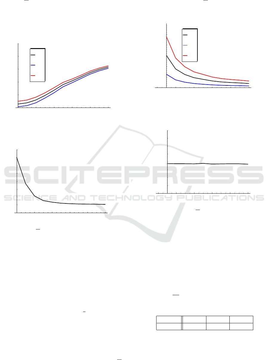
This effect is visible clearly in Fig. 4, in which
the ratio
L
2
L
1
is depicted as a function of D(F). As
we may notice, L
2
is about 7 times larger than L
1
,
when D(F) is small. But the difference diminishes,
as D(F) grows, and for D(F) = 10, both L
2
and L
1
are practically the same.
2 4 6 8 10
DHFL
0.1
0.2
0.3
0.4
0.5
Loss ratio
L
2
L
1
L
Figure 3: Dependence of the total and per-flow loss ratios
on the standard deviation of the service time.
2 4 6 8 10
DHFL
1
2
3
4
5
6
7
8
L
2

L
1
Figure 4: Ratio
L
2
L
1
versus the standard deviation of the ser-
vice time.
4.6 Dependence on the Buffer Size
In all the previous experiments, we did not change
the buffer size. In the next scenario, we varied the
buffer size from 10 to 100 and observed, how this
affects the per-flow loss ratios and their relations to
each other. We used again two flows which had very
different their own standard deviations, to see this
time how the buffer size affects such different flows.
Namely, it was N = 2, λ
1
= λ
2
=
1
2
, G
1
was uniform
on the interval (1,3), G
2
was Γ(0.16,12.5), and we
had D(G
1
) = 0.577, D(G
2
) = 5.
The results are depicted in Fig. 5. All three loss
ratios decrease with time, which is not surprising.
However, the relation between L
1
and L
2
is quite dif-
ferent than the one observed in the previous experi-
ment. It can be seen in Fig. 6, in which the ratio
L
2
L
1
is
depicted for various buffer sizes. For two quite differ-
ent flows, the proportion
L
2
L
1
is virtually the same for
the buffer sizes which differ by an order of magnitude.
0 20 40 60 80 100
b
0.05
0.1
0.15
0.2
0.25
Loss ratio
L
2
L
1
L
Figure 5: Dependence of the total and per-flow loss ratios
on the buffer size.
0 20 40 60 80 100
b
1
2
3
4
5
6
7
8
L
2

L
1
Figure 6: Ratio
L
2
L
1
versus the buffer size.
4.7 Special Case: Poisson Flows Only
In subsection 4.2 we showed simulation results, in
which the per-flow loss ratios were different, even
though all the flows had the same type of the inter-
arrival time distribution (but the rates were different).
In the following experiment, we checked if this
holds true if all the flows are Poisson. Namely, the
following parameters were used: N = 3, all interar-
rival times exponential, with the average values of
100, 10 and
100
89
in different flows, respectively. The
rates were thus λ
1
= 0.01, λ
2
= 0.1 and λ
3
= 0.89, the
buffer size was 50. The obtained results are:
L L
1
L
2
L
3
0.0195 0.0194 0.0195 0.0195
As we can see, all the per-flow loss ratios are the
same now. This observation, which differs from the
one of subsection 4.2, is most likely caused by the
special properties of the Poisson process and expo-
QQSS 2021 - Special Session on Quality of Service and Quality of Experience in Systems and Services
626

nential distribution. As we know, a superposition of
many Poisson processes, perhaps of different rates, is
again a Piosson processes. This is a consequence of
the memoryless property of the exponential distribu-
tion, which is the only one among continuous distri-
bution possessing this property.
5 CONCLUSIONS
In this paper, we presented a simulation study of the
per-flow loss ratios caused by an overflowed buffer
at the output interface of a networking device. We
tried to find the properties of the flow that may in-
fluence its loss ratio, investigated the possible mutual
dependencies between the flows, studied the impact
of the buffer size and the distribution of the service
time (packet size) on the per-flow loss ratios, as well
as their relations to ech other. Several interesting ob-
servations were made in the simulations. In particular,
we observed that:
• the per-flow loss ratios were different from each
other and different from the total loss ratio, even
when the flows had the same type of the interar-
rival time distribution, but different rates;
• the per-flow loss ratios were different from each
other and different from the total loss ratio, even
when the flows had the same rates, but different
interarrival time distributions;
• the per-flow loss ratio of a particular flow, as well
as the total loss ratio, grew with the standard devi-
ation of that flow, while the losses of other flows
were practically unaffected;
• the per-flow loss ratios and the total loss ratio
grew with the standard deviation of the service
time;
• as the standard deviation of the service time grew,
the differences between the per-flow loss ratios
got smaller, even for flows of quite different types.
For a large standard deviation of the service time,
these differences practically vanished;
• the per-flow loss ratios decreased with the buffer
size, but the proportions between them were
maintained, i.e. different buffers affected the per-
flow loss ratios in the same way, even if the flows
were of very different types;
• the per-flow loss ratios were all the same only in
two cases: when all the flows had the same inter-
arrval time distributions and rates, or when all the
flows had the exponential interarrvial time distri-
bution (in the latter case, the rates might not be
the same).
As for the future work, it would be great if we
could solve analytically the model presented in Sec-
tion 2, so that all the results and conclusion obtained
here via simulations could be obtained from formu-
las. Unfortunately, this seems to be far beyond the
state of the art of the queueing theory. The model
considered herein, is clearly a generalization of the
classic G/G/1/b model, i.e. we can obtain the G/G/1/b
model by putting N = 1 to the model of Section 2.
It is well known, however, that the exact solution of
the G/G/1/b is very hard to obtain, and nobody have
succeeded so far in finding it. Naturally, solving the
model of Section 2 would be even harder.
Therefore, we are left with the following two pos-
sibilities. Firstly, we can restrict the analysis to some
special cases of the model, for instance to some spe-
cial distributions of the interarrival time. The G/G/1/b
model has several know solutions for special distri-
butions, like exponential, Erlang and other Marko-
vian distributions. Secondly, we may search for ap-
proximate solutions of the model of Section 2. There
are many successful approaches to solve the G/G/1/b
model approximately, so maybe the same is possible
in the case of the multi-flow arrival model.
Finally, it is recommended by Internet Engineer-
ing Task Force, (Baker and Fairhurst, 2015), that the
classic finite-buffer queueing at routers’ output inter-
faces are replaced by some active queue management
algorithms (Chrost et al., 2009; Chrost and Chydzin-
ski, 2013). In these algorithms, the losses occur be-
fore the buffer gets full and are caused by the algo-
rithm itself. It would be interesting to extend to the
per-flow loss analysis to models of such algorithms
(Chydzinski and Mrozowski, 2016).
ACKNOWLEDGEMENTS
This work was conducted within project
2020/39/B/ST6/00224, founded by National Science
Centre, Poland.
REFERENCES
Baker, F. and Fairhurst, G. (2015). Ietf recommendations
regarding active queue management. In Request for
Comments 7567.
Benko, P. and Veres, A. (2002). A passive method for es-
timating end-to-end tcp packet loss. In Proc. of IEEE
GLOBECOM, pages 2609–2613.
Bolot, J.-C. (1993). End-to-end packet delay and loss be-
havior in the internet. In Conference Proceedings on
Communications Architectures, Protocols and Appli-
cations, pages 289–298.
Per-flow Packet Loss Ratios Induced by an Overflowed Buffer
627

Bratiychuk, M. and Chydzinski, A. (2009). On the loss pro-
cess in a batch arrival queue. Applied Mathematical
Modelling, 33(9):3565–3577.
Chrost, L., Brachman, A., and Chydzinski, A. (2009). On
the performance of aqm algorithms with small buffers.
Communications in Computer and Information Sci-
ence, 39:168–173.
Chrost, L. and Chydzinski, A. (2013). On the deterministic
approach to active queue management. Telecommuni-
cation Systems, 63(1):27–44.
Chydzinski, A. and Adamczyk, B. (2012). Transient and
stationary losses in a finite-buffer queue with batch
arrivals. Mathematical Problems in Engineering,
2012:1–17.
Chydzinski, A. and Mrozowski, P. (2016). Queues with
dropping functions and general arrival processes.
PLoS ONE, 11(3):1–23.
Chydzinski, A. and Samociuk, D. (2019). Burst ratio in
a single-server queue. Telecommunication Systems,
70(2):263–276.
Chydzinski, A., Samociuk, D., and Adamczyk, B. (2018).
Burst ratio in the finite-buffer queue with batch pois-
son arrivals. Applied Mathematics and Computation,
330:225–238.
Chydzinski, A., Wojcicki, R., and Hryn, G. (2007). On the
number of losses in an mmpp queue. In Next Gen-
eration Teletraffic and Wired/Wireless Advanced Net-
working, pages 38–48. Springer Berlin Heidelberg.
Cidon, I., Khamisy, A., and Sidi, M. (1993). Analysis of
packet loss processes in high-speed networks. IEEE
Transactions on Information Theory, 39(1):98–108.
Coates, M. and Nowak, R. (2000). Network loss inference
using unicast end-to-end measurement. In Proc. of
ITC Conference on IP Traffic, Measurement and Mod-
eling, pages 282–289.
Duffield, N., Lo Presti, F., Paxson, V., and Towsley, D.
(2001). Inferring link loss using striped unicast
probes. In Proc. of IEEE INFOCOM, pages 915–923.
Hasslinger, G. and Hohlfeld, O. (2008). The gilbert-elliott
model for packet loss in real time services on the inter-
net. In 14th GI/ITG Conference - Measurement, Mod-
elling and Evalutation of Computer and Communica-
tion Systems, pages 1–15.
McGowan, J. W. (2005). Burst ratio: a measure of
bursty loss on packet-based networks. In US Patent
6,931,017.
Rachwalski, J. and Papir, Z. (2014). Burst ratio in concate-
nated markov-based channels. Journal of Telecommu-
nications and Information Technology, 1:3–9.
Rachwalski, J. and Papir, Z. (2015). Analysis of burst ratio
in concatenated channels. Journal of Telecommunica-
tions and Information Technology, 4:65–73.
Salvador, P., Valadas, R., and Pacheco, A. (2003). Multi-
scale fitting procedure using markov modulated pois-
son processes. Telecommunication Systems, 23(1-
2):123–148.
Samociuk, D. and Barczyk, M.and Chydzinski, A. (2019).
Measuring and analyzing the burst ratio in ip traf-
fic. Lecture Notes of the Institute for Computer
Sciences, Social Informatics and Telecommunications
Engineering, 303:86–101.
Samociuk, D., Chydzinski, A., and Barczyk, M. (2018). Ex-
perimental measurements of the packet burst ratio pa-
rameter. Communications in Computer and Informa-
tion Science, 928:455–466.
Sanneck, H. and Carle, G. (1999). Framework model
for packet loss metrics based on loss runlengths. In
Multimedia Computing and Networking 2000, volume
3969.
Sommers, J., Barford, P., Duffield, N., and Ron, A. (2005).
Improving accuracy in end-to-end packet loss mea-
surement. ACM SIGCOMM Computer Communica-
tion Review, 35(4):157–168.
Takagi, H. (1993). Queueing analysis - Finite Systems.
North-Holland, Amsterdam.
Yajnik, M., Moon, S., Kurose, J., and Towsley, D. (1999).
Measurement and modelling of the temporal depen-
dence in packet loss. In IEEE INFOCOM ’99. Con-
ference on Computer Communications. Proceedings.
Eighteenth Annual Joint Conference of the IEEE Com-
puter and Communications Societies. The Future is
Now (Cat. No.99CH36320), volume 1, pages 345–
352.
Yoshihara, T., Kasahara, S., and Takahashi, Y. (2001).
Practical time-scale fitting of self-similar traffic with
markov-modulated poisson process. Telecommunica-
tion Systems, 17(1/2):185–211.
Yu, X., Modestino, J., and Tian, X. (2005). The accuracy
of gilbert models in predicting packet-loss statistics
for a single-multiplexer network model. In Proceed-
ings IEEE 24th Annual Joint Conference of the IEEE
Computer and Communications Societies., volume 4,
pages 2602–2612.
QQSS 2021 - Special Session on Quality of Service and Quality of Experience in Systems and Services
628