Manipulating Deformable Objects with a Dual-arm Robot

ephane Caro

1 a

, Christine Chevallereau

1 b

and Alberto Remus

Centre National de la Recherche Scientiﬁque (CNRS), Laboratoire des Sciences du Num

erique de Nantes (LS2N),

44300 Nantes, France

Ecole Centrale de Nantes, 44300 Nantes, France

Keywords:

Deformable Models, Dual-arm Robot, Manipulation, Stability Analysis.

Abstract:

Competition in all sectors requires companies to be increasingly ﬂexible to market changes and the assembly

industry is no exception. The impact of this work concerns aircraft production, as well as other ﬁelds. The

main focus is on modelling and control techniques to carry out assembly tasks involving deformable parts, by

exploiting a multi-robot system. Speciﬁcally, two robot arms are used to move a light and deformable part in

order to adapt its shape for an assembly operation. A vision system is used, assisted by markers. Furthermore,

the stability of the proposed controller is analyzed and experimental results are given.

1 INTRODUCTION

Assembly process is one of the cornerstones of in-

dustry because it allows to couple parts together

in order to get a sub-product or a ﬁnished product

(Marvel et al. (2018)). This work investigates the

added value brought by a robotic system composed

by robots, which have to cooperate in order to per-

form an assembly task involving deformable objects.

Manipulation of ﬂexible objects has been consid-

ered in prior work with different control approaches

such as impedance control (Sun and Liu (1997))

and (Erhart and Hirche (2013)), force control (Sun

and Liu (2001)) or sliding mode control (Tavasoli

et al. (2009)). Visual approaches have also been

used in several studies (Smolen and Patriciu (2009)),

(Hirai and Wada (2000)),(Wada et al. (2001)) us-

ing a theoretical model of the object deformation

or with an adaptive model of deformation built on-

line (Navarro-Alarcon et al. (2016)). Here a visual

approach is investigated as well, but a constant model

of the beam deformation is used since the results

of stability analysis show that an adaptive model is

not required to manipulate the object at hand. Sev-

eral papers are dedicated to more compliant objects

such as tissues (Berenson (2013); Jia et al. (2018)).

Under some assumptions, many parts to be assem-

bled in industry can be modelled as planar ﬂexible

beams (Bertelsmeier et al. (2017)) and this greatly

https://orcid.org/0000-0002-8736-7870

https://orcid.org/0000-0002-1929-5211

simpliﬁes the modelling and control, which is com-

mon in industry like aircraft production (Al-Yahmadi

and Hsia (2007)). To reproduce an assembly task,

the work cell used in the framework of this research

work is endowed with a ﬁxture coupled to a ﬂexible

beam. A new modelling technique is presented based

on the elastic properties of the beam, which can be ex-

ploited to measure its deformation. The control aspect

and the use of vision are essential because of the un-

certainties in the ﬂexible object modelling (Navarro-

Alarcon et al. (2016)).

Several robots cooperating and manipulating the

same object amount to a closed-loop mechanism with

a deformable beam. Such a system is under-actuated

due the inﬁnite number of degrees of freedom induced

by the ﬂexible beam. Here some key points are lo-

cated on the beam to ease the control of the over-

all system. Contrary to methods that use a phys-

ical model of the deformable object and its stable

equilibrium (Bretl and McCarthy (2014)),(Sintov et

al. (2020)), very simple deformation models adapted

to our control strategy will be used. Moreover, this

ﬁrst-order model can be built experimentally based on

visual information.

The main contribution of this paper, essentially

methodological, lies in the use of the model estima-

tion for the motion control of a deformable beam and

the stability analysis of the proposed controlled law. It

should be noted that the proposed approach is based

on a classical position control available on all indus-

trial robots, and a high level loop based on vision

Caro, S., Chevallereau, C. and Remus, A.

Manipulating Deformable Objects with a Dual-arm Robot.

DOI: 10.5220/0010707600003061

In Proceedings of the 2nd International Conference on Robotics, Computer Vision and Intelligent Systems (ROBOVIS 2021), pages 48-56

ISBN: 978-989-758-537-1

feedback. The approach does not require force mea-

surement or force control. Besides, it is simpler than

the one introduced in (Navarro-Alarcon et al. (2016))

because it is based on a non-adaptive model and

deﬁned from the desired object pose thanks to a

detailed stability analysis. Furthermore, it is well

suited to industrial applications and manipulation of

large objects, but less ﬂexible than those considered

in (Navarro-Alarcon et al. (2016)) and (Lagneau et

al. (2020)).

The paper is organized as follows. Section 2

presents the experimental setup and its parameteriza-

tion. Section 3 introduces the kinematic sensitivity

Jacobian matrix associated with the beam shaping and

displacement in a plane. Section 4 describes the pro-

posed control law of the dual-arm robot and its per-

formance in terms of stability and accuracy. Finally,

conclusions are drawn in Section 5.

2 EXPERIMENTAL SETUP

The section describes the robotic cell and its main

components used in the framework of the research

work presented in the paper. Besides, a simpliﬁed

model of the multi-robot system and the four spaces

at stake used for its control are explained.

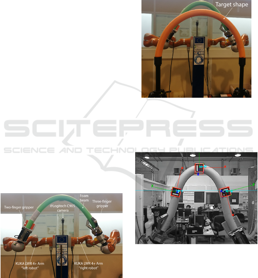
As shown in Figs. 1 and 2, the experimental setup

located at LS2N is composed of (i) two KUKA LWR

4+ 7-dof robotic arms, the left one being endowed

with a two-ﬁngers gripper and the right one being

equipped with a three-ﬁngers hand; (ii) one ﬂexible

beam; (iii) one target, named target shape, for the

beam; (iv) one ®Logitech C905 camera, which is

used as a detection system to extract keypoints from

both the beam and the target shape.

Figure 1: A ﬂexible beam grasped by two KUKA LWR 4+

7-dof robotic arms.

The two robots are position-based controlled.

Contrary to the geometric and kinematic models of

the robots, the model of the ﬂexible beam is not

known beforehand. Therefore, a technique to obtain

this model is described in this paper based on some

ArUco Markers (Garrido-Jurado et al. (2014)) stuck

on the beam as illustrated in Fig. 3. The shape and

Figure 2: Target shape for the ﬂexible beam.

position of the target shape are supposed to be still in

the workcell. Note that the ﬂexible beam is initially

positioned by a human operator, due to the complexity

of the automatic detection and grasping of the ﬂexible

beam.

Figure 3: Three ArUco Markers stuck on the ﬂexible

beam and detected by a ®Logitech C905 camera through

OpenCV.

2.1 The Multi-robot System

The two serial robots and the ﬂexible beam can be

seen as a planar closed-loop mechanism, which is in-

trinsically under-actuated due to the inﬁnite number

Manipulating Deformable Objects with a Dual-arm Robot

of degrees of freedom provided by the ﬂexible beam

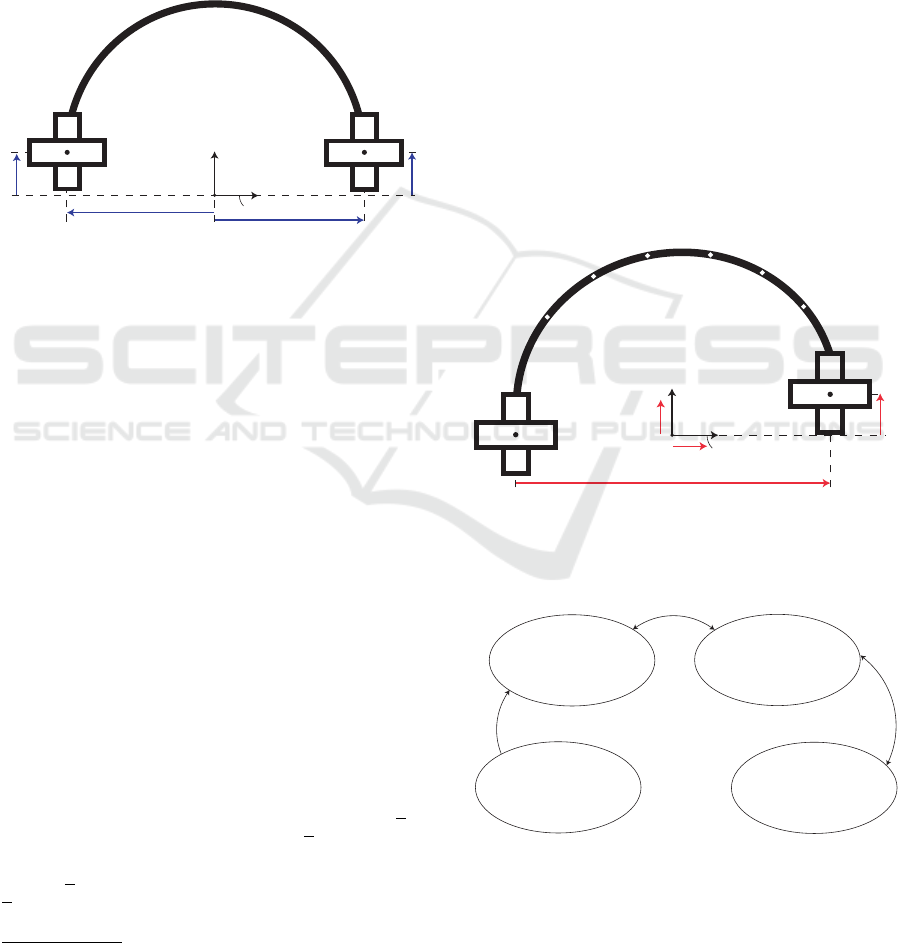
as depicted in Fig. 4. Without loss of generality, the

beam and its attachement points E

and E

with the

grippers are supposed to move in the plane passing

through point O and normal to x

, x

being normal

to both axes y

and z

. Thus, the beam does not

twist during its positioning and shaping in the base

frame F

of origin O and axes y

and z

. The planar

displacement of the left (right, resp.) robot is param-

eterized by the Cartesian coordinates y

and z

and

, resp.) of point E

, resp.) expressed in F

Left robot

Right robot

Figure 4: Planar closed-loop mechanism composed of a

ﬂexible beam and two grippers.

The robots are assumed to behave like rigid sys-

tems with regard to the beam, the latter being much

more ﬂexible. As a consequence, variables y

, z

and z

should be controlled to position and shape

the ﬂexible beam in order to superimpose it the tar-

get shape for the beam shown in Fig. 2. Therefore,

a modelling and control strategy of the ﬂexible beam

should ﬁrst be developed based on the location of the

ArUco Markers expressed in F

and detected by the

®Logitech C905 camera.

2.2 Four Spaces

In order to reach its target shape shown in Fig. 2, the

ﬂexible beam is deformed and displaced by the two

KUKA LWR 4+ 7-dof robotic arms, named left and

right robots respectively in what remains, endowed

with their own gripper as shown in Fig.1. It is note-

worthy that four spaces are at stake to deform and

move the beam in F

. Those four spaces are deﬁned

as follows: (i) the robots joint space (R J S ) is the set

of robot revolute joint variables, namely,

R J S = {q = [... q

i j

.. .]

∈ R

: q

i j

≤ q

i j

≤ q

i j

i = l,r , j = 1,...,7} (1)

i j

and q

i j

being the lower and upper bounds of rev-

olute joint angle q

i j

and are given in

. l and r

https://www.kuka.com/en-de/products/robot-systems/

industrial-robots/lbr-iiwa

stand for the left and right robots, resp.; (ii) the end-

effector space (EES) is the set Cartesian coordinates

of points E

and E

expressed in F

satisfying the pla-

nar closed-loop shown in Fig. 4, namely,

EES = {p = [y

]

∈ R

− y

)

+ (z

− z

)

≤ l

} (2)

being the length of the ﬂexible beam; (iii) the de-

formation input space (DI S ) is the set of variables

associated to the positioning and shaping of the beam:

DI S = {u = [y

]

∈ R

: (5a)-(d) are satisﬁed}

(3)

variables y

, z

, y

, z

being depicted in Fig. 5;

(iv) the keypoint space (K S ) deﬁnes the location of

the ArUco Markers stuck on the ﬂexible beam, i.e.,

K S = {x = [y

.. .y

]

∈ R

} (4)

and z

being the Cartesian coordinates of key-

point P

expressed in F

, k = 1, .. .,N with N the num-

ber of keypoints as shown in Fig. 5.

Left robot

Right robot

)

Figure 5: Variables associated with DI S and K S .

The relationships between the four spaces are rep-

resented in Fig. 6.

Robots Joint Space

{q =[...q

...]

∈ R

}

End-Eﬀector Space

{p =[y

]

∈ R

}

Deformation Input Space

{u =[y

]

∈ R

}

Keypoint Space

{x =[y

...y

]

∈ R

}

DGM

Eqs. (5a)-(d)

Flexible beam

sensitivity Jacobian

matrix – Eq. (6)

Figure 6: Relationship between the robots joint, end-

effector, deformation input and keypoint spaces.

ROBOVIS 2021 - 2nd International Conference on Robotics, Computer Vision and Intelligent Systems

3 BEAM DEFORMATION

The beam is displaced and shaped by controlling the

overall system in DI S. From Figs. 4 and 5, the vari-

ables y

, z

devoted to the positioning of the beam

in F

and the variables y

, z

related to its shaping

are deﬁned as a function of Cartesian coordinates of

points E

and E

as follows:

= y

− y

(5a)

= z

− z

(5b)

= (y

+ y

)/2 (5c)

= (z

+ z

)/2 (5d)

It should be noted that the precision of the beam mod-

eling from the keypoint detection is a function of N.

The higher N, the better the precision. The maximum

number of keypoints to avoid an under-actuated sys-

tem is two. Indeed, if N = 2, the system will have as

many input variables as ouput variables. On the con-

trary, the number of input variables is lower than the

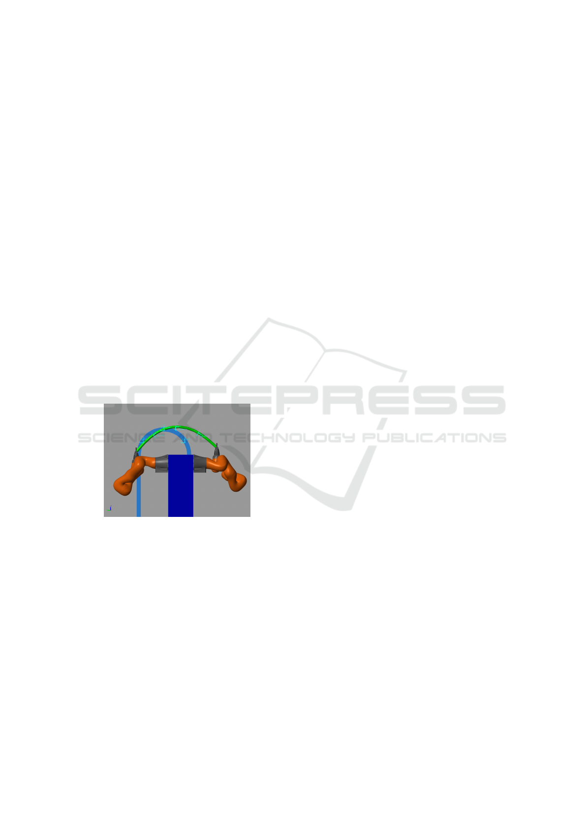
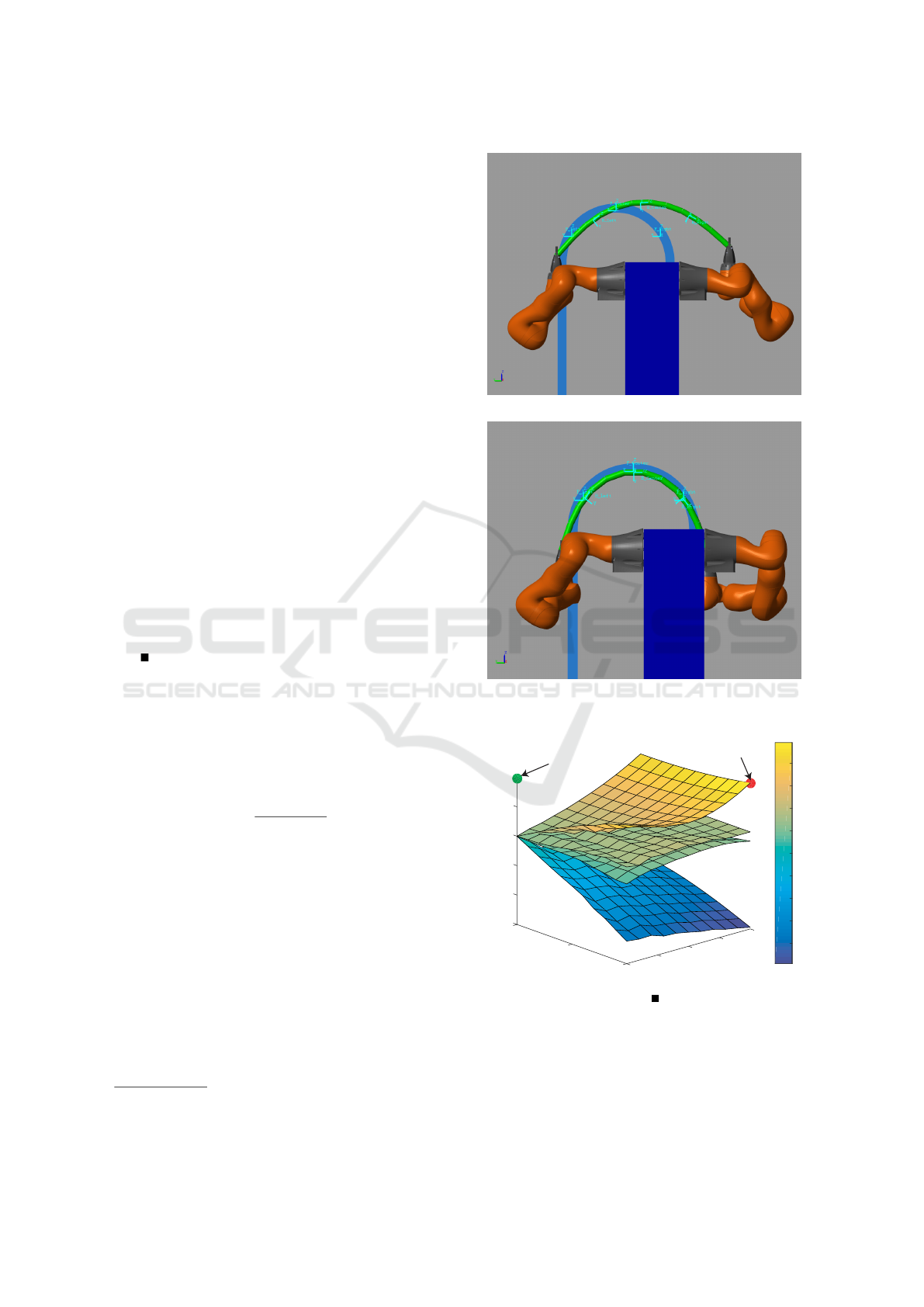
number of output variables, i.e., 2N, when N > 2. Fig-

ure 7 shows an example of a simulated under-actuated

system where with three keypoints are located both on

the beam and its target shape. Note that each keypoint

on the beam is assigned to its own keypoint on the tar-

get shape.

Figure 7: Three keypoints located both on the beam and its

target shape: the system is under-actuated.

3.1 Sensitivity Matrix

The variation δx in keypoint vector x, deﬁned in (4),

can be expressed as a function of the variation δu in

input variable vector u, deﬁned in (3), as follows:

δx = J(y

)δu (6)

where J is a (2N × 4)-sensitivity Jacobian matrix, as

in (Caro et al. (2009)), taking the form:

J =





(7)

δy

and δz

correspond to a small displacement of the

whole beam, thus they affect the displacement of all

the keypoints with the same manner. However, they

do not affect the shape of the beam. Thus, the last two

columns j

and j

of matrix J are expressed as:



1 0 1 0 .. . 1 0



(8)



0 1 0 1 .. . 0 1



(9)

and j

are the ﬁrst two columns of matrix J

and two 2N-dimensional vectors taking the form:



.. . δy

/δy

δz

/δy

.. .



(10)



.. . δy

/δz

δz

/δz

.. .



(11)

with k = 1,. .. ,N. δy

/δy

(δz

/δy

, resp.) denotes

the sensitivity of coordinate y

, resp.) to varia-

tion δy

in variable y

. δy

/δz

(δz

/δz

, resp.) de-

notes the sensitivity of coordinate y

, resp.) to

variation δz

in variable z

. Those sensitivity coef-

ﬁcients are not a function of variables y

and z

The terms of the ﬁrst two column vectors j

and j

of matrix J are identiﬁed either in simula-

tion as explained in Sec. 3.2 or experimentally as de-

scribed in Sec. 3.3 for a given shape of the beam,

i.e., for given y

and z

nominal values. The iden-

tiﬁcation methodology aims at measuring the point-

displacements of keypoints P

, k = 1, .. ., N, namely,

the variations δy

and δz

in their Cartesian coordi-

nates for several small variations δy

and δz

3.2 Simulation

The robotic platform shown in Fig. 1 was simulated

thanks to Simscape Multibody

and Simulink

deal with modelling, control and visualization. The

beam was modeled based on the lumped parameters

method presented in (Miller et al. (2006)). The beam

was discretized in twelve mass unit, linked together

by revolutes joint endowed with a certain stiffness and

damping, whose parameters depend on the material

used. As far as the foam beam depicted in Fig. 1 is

concerned, its length l

and diameter d

are equal to

1.14 m and 0.064 m, respectively. The Young’s modu-

lus E and density ρ of the foam are equal to 0.005 GPa

and 50 kg/m

, respectively.

In what remains, three keypoints are supposed to

be equally spaced on the beam, i.e. N = 3, to match

with the three ArUco Markers shown in Fig. 3.

Figure 8 shows the variations δz

, δz

and δz

in the z-coordinates of points P

, P

and P

associ-

ated with small variations δy

as a function of y

, y

varying from 0.8 m to 1 m. It is apparent that the

higher y

, i.e., the larger the distance points E

and E

the more sensitive the z-coordinates of the keypoints

to small variations in y

. Besides, the z-coordinate of

the mid-keypoint P

is more sensitive to δy

than the

z-coordinates of the lateral keypoints P

and P

. The

Manipulating Deformable Objects with a Dual-arm Robot

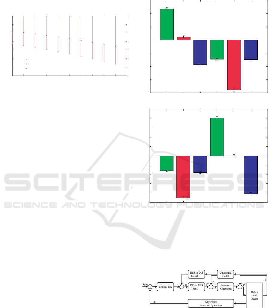
plots corresponding to P

and P

overlap because the

last two keypoints have the same sensitivity to δy

δz

/δy

δz

/δy

δz

/δy

0.82

0.86

0.9 0.94 0.98

-0.1

-0.2

-0.3

-0.4

-0.5

-0.6

-0.7

δz

/δy

[]

[m]

Figure 8: Sensitivity of the z-coordinates of keypoints P

and P

to small variations in y

obtained from simulation.

3.3 Experiments

As explained in Sec. 3.1, the terms of matrix J can

also be identiﬁed experimentally. Experiments were

carried out by gluing three ArUco Markers on the

foam beam as illustrated in Fig. 3 and by using a cal-

ibrated monocular camera to detect them. Robot Op-

erating System was used to control the robots.

Twenty tests were performed per set of y

and

nominal values to determine the mean and stan-

dard deviation of the sensitivity coefﬁcients δy

/δy

δz

/δy

, δy

/δz

and δz

/δz

, k = 1,2,3. Figure 9

highlights the mean values of those coefﬁcients for

= 0.8 m and z

= 0 m. Furthermore, Fig. 9 shows

the conﬁdence intervals associated with the forego-

ing sensitivity coefﬁcients and assessed experimen-

tally by considering the following sources of errors:

(i) camera calibration and placement errors; (ii) un-

certainties in the beam grasping; (iii) bad knowledge

of the beam characteristics; (iv) vibrations of the key-

points and slight scattering during trajectory execu-

tion.

It should be noted that the sensitiviy coefﬁcients

identiﬁed experimentally differ slightly from the sim-

ulation results shown in Fig. 8. More conﬁdence can

be given to experimental results because the conﬁ-

dence intervals are quite small and the uncertainties in

the experimental setup and in the ﬂexible beam model

are difﬁcult to take into account in simulation.

4 CONTROL LAW

The objective of the control law is to bring the ArUco

Markers, i.e. the keypoints, stuck on the ﬂexible

beam, as shown in Fig. 3, in front of the markers glued

on the target shape illustrated in Fig. 2. The closed

loop control law that deﬁnes the displacement of end-

δy

/δy

δy

/δy

δy

/δy

δz

/δy

δz

/δy

δz

/δy

0.3

0.2

0.1

-0.1

-0.2

-0.3

-0.4

(a)

δy

/δz

δy

/δz

δy

/δz

δz

/δz

δz

/δz

δz

/δz

0.3

0.2

0.1

-0.1

-0.2

-0.3

-0.4

0.4

(b)

Figure 9: Experimental mean values and conﬁdence in-

tervals associated with the terms of (a) j

and (b) j

for

= 0.8 m and z

= 0 m.

effectors E

and E

in DI S is described in this section.

Then classical control of the robot is used with a low

level control in R J S as shown in Fig. 10.

(5)

Figure 10: Overall control scheme for position and shape

control.

The desired end-effector pose vector p is ex-

pressed from the deformation input vector u by

Eqs. (5a)-(d). Note that the KUKA LWR 4+ robotic

arm is kinematically redundant because it has seven

revolute joints. Therefore, the Moore-Penrose inverse

of the kinematic Jacobian matrix of each robotics

ROBOVIS 2021 - 2nd International Conference on Robotics, Computer Vision and Intelligent Systems

arm is used to compute δq, the variation in revolute

joint angle vector q as a function of a small displace-

ment δp of end-effectors E

and E

in F

. Then the

desired revolute joint angle vector q is deduced and

sent to the low level controller of the robot.

The control law used to deﬁne vector u is based on

visual servoing control in the task space (Chaumette

et al. (1991)). It should be noted that the sensitivity

Jacobian matrix (7) amounts to an interaction matrix.

From Eq. (7), the end-effector velocity

x is expressed

as a function of the time derivative

u of vector u as

follows:

x = J

u (12)

with x being deﬁned in (4). Let x

des

denote the desired

keypoints coordinate vector expressed in F

. Thus,

the error e in K S takes the form:

e = x − x

des

(13)

The following equation should be met for e to de-

crease with an exponential rate:

e = −λe (14)

with λ being a positive gain and

e the time deriva-

tive of e. By substituting (13) into (14) and assuming

that x

des

is constant, we get:

x = −λ(x − x

des

) (15)

Since the relation between x and u is not known,

it is estimated as,

x =

u (16)

By combining (15) and (16) we obtain:

u = −λ

(x − x

des

) (17)

with

being the Moore–Penrose inverse of the es-

timated sensitivity Jacobian matrix

J. From (6), J is

a function of u. It means that several estimated ma-

trix

J can be found. Here, the used estimated sen-

sitivity matrix named

∗

is the matrix J assessed at

the ﬁnal desired conﬁguration u

of the beam, i.e., for

= 0.8 m and z

= 0 m. It will be shown in Sec. 4.2

that this choice is relevant in terms of control stability.

As a result, the control law is:

u = −λ

∗

(x − x

des

) (18)

Note that (18) provides a velocity in DI S whereas

the control law requires the variation δu. As a con-

sequence, a duration t

of motion is deﬁned and the

control law becomes:

δu = −λt

∗

(x − x

des

) (19)

Note that t

is about twenty times the sampling period,

the latter equals 5 ms, of the low level control of the

KUKA LWR 4+ robotic arms.

4.1 Stability Analysis

The stability analysis is useful to understand at ﬁrst

glance the performance of the control law. First, a

Lyapunov function L based on the tracking error is

deﬁned to study the stability:

L =

e (20)

The derivative of L is:

L = e

e (21)

Since the desired position and shape of the beam are

ﬁxed, the evolution of the error

e as function of the

control input can be expressed as:

e =

x = J(u)

u (22)

With the proposed control law (18),

e takes the form:

e = −λJ(u)

∗

e (23)

Using (23) in (21), we obtain

L = −λe

J(u)

∗

e (24)

If the matrix J(u)

∗

is positive deﬁnite, the conver-

gence of e to zero will be insured. However this ma-

trix is a (2N × 2N)-matrix of rank ≤ 4. Thus this con-

dition cannot be met when N > 2.

It should be noted that if

∗

e = 0, i.e., if x−x

des

in the kernel of

∗

, then the

u command will be null

and the error e will not be reduced but will remain

constant. Knowing that the ﬁnal error cannot always

be null since N ≥ 3 control points are used for four

available commands only, the evolution of the error

projected in the image of

∗

is studied. Accordingly,

a new four-dimensional error vector  is deﬁned as

follows:

 =

∗

e (25)

The evolution of  can be deduced by time derivation

of (25), namely,

˙ =

∗

e (26)

since

∗

is a constant matrix. Using (23), and (25), ˙

can be expressed as:

˙ = −λ

∗

J(u) (27)

From (27), a sufﬁcient condition to ensure the sys-

tem stability is the matrix

∗

J(u) to be positive deﬁ-

nite (Zake et al. (2019a); Zake et al. (2019b)). Since

∗

J(u) may not be symmetric, its deﬁnite positive-

ness is analyzed based on the eigenvalues of its asso-

ciated symmetric matrix . As a result, a sufﬁcient

condition to ensure the system stability becomes:

= 1/2(

∗

J(u))

+ 1/2(

∗

J(u)) > 0,∀t (28)

Manipulating Deformable Objects with a Dual-arm Robot

Indeed, if this condition is satisﬁed, the error ˙ will

always decrease to ﬁnally reach 0. The results on lo-

cal stability of the proposed control law are given in

Sec. 4.2.

As far as the ﬁnal error is concerned, if the posi-

tion x

des

of the target markers and the position x of

the markers stuck the beam are such that moving one

of the robot end-effectors to reduce a distance for one

marker to its target leads to an increase of a distance

from another marker to its own target, the controller

will have better do nothing. From (6), only the error

x −x

des

that belongs to the image of J can be reduced

by the control input. The part of the error that is in

the kernel of J(u)

cannot be cancelled. Since the

proposed control law is built based on sensitivity ma-

trix J estimated at the expected ﬁnal pose and shape

of the beam, it leads to the smallest ﬁnal error.

4.2 Simulation

The aforementioned method can be implemented by

means of Simscape Multibody

and Simulink

The control law minimizes the error between each

keypoint on the beam and its assigned marker on the

target shape as shown in Fig. 11 while considering

large position errors for the keypoints at the start con-

ﬁguration.

Figure 12 shows that the four eigenvalues of ma-

trix are positive within the intervals 0.8 m < y

1 m and −0.2 m < z

< 0 m. From (28), the system

will be stable for any initial conﬁguration (y

)

taken in those intervals with the ﬁnal conﬁguration

d f

) = (0.8 m,0 m).

In addition to stability analysis, the error ξ in K S

is considered as another performance index of control

law (18). ξ is the root-mean square error of the key-

point position:

ξ =

||x − x

des

/N (29)

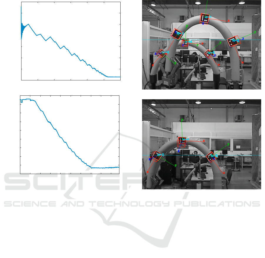
Figure 13(a) shows the evolution of ξ with time

for the simulated system, N = 3. ξ decreases and sta-

bilizes at a small value as expected.

4.3 Experiments

Figure 14 and video

represent the task performed ex-

perimentally thanks to control law (18). The corre-

sponding values of ξ deﬁned in (29) are depicted in

Fig. 13b. The experimental decrease of ξ is slower

than the simulated one because of the slow detection

of the ArUco markers by the low-cost camera used

and vibrations.

https://uncloud.univ-nantes.fr/index.php/s/

kZpNNAQ98PpBr9C

(a)

(b)

Figure 11: Start (a) and end (b) of the task in simulation.

0.7

0.8

0.9

1.1

0.95

1.2

-0.1

0.9

0.85

-0.2

0.8

0.75

0.8

0.85

0.9

0.95

1.05

1.1

1.15

[m]

Eigenvalues of Π

End conﬁg.

Start conﬁg.

Figure 12: The eigenvalues of as a function of y

and z

ROBOVIS 2021 - 2nd International Conference on Robotics, Computer Vision and Intelligent Systems

0.14

0.12

0.1

0.08

0.06

0.04

0.02

time [s]

ξ [m]

(a)

time [s]

0.18

0.16

0.14

0.12

0.1

0.08

0.06

0.04

0.02

ξ [m]

(b)

Figure 13: Root-mean square error of the keypoint position:

(a) simulation; (b) experiments.

5 CONCLUSIONS AND FUTURE

WORK

This paper dealt with a control law for manipulating

a ﬂexible beam with a dual-arm robot. The approach

is characterized by the fact that a deformation model

of the object is not necessary since it is experimen-

tally constructed. This will be particularly useful if

the material is anisotropic or poorly identiﬁed. The

built model is adapted to the proposed control law be-

cause the elastic deformations induced by the beam

deformation provided by the robots are measured. A

fairly complete simulation study showed that it is pos-

sible to only use the deformation model of the ﬂexible

object corresponding to its intended conﬁguration for

manipulation by ensuring the stability of the control

through the whole task. Accordingly, an online esti-

mation as proposed in (Navarro-Alarcon et al. (2016))

is not required with the control approach presented in

this paper. Indeed an acceptable deformation model

of the beam is constructed experimentally. The contri-

bution of the paper is essentially methodological and

the results are illustrated with the planar deformation

(a)

(b)

Figure 14: Start (a) and end (b) of the task experimentally.

of a beam using markers. Later on, the proposed ap-

proach will be extended to the positioning, shaping

and assembling of three-dimensional ﬂexible objects

with more than two robotic arms. The online detec-

tion of the beam deformation was performed thanks to

some markers as a proof of concept. Such a detection

can be extended by using points of interest extracted

from images.

REFERENCES

J. Marvel, R. Bostelman, and J. Falco, Multi-Robot As-

sembly Strategies and Metrics, ACM Comput Surv.,

vol. 51(1), 2018. doi: 10.1145/3150225.

D. Sun, Y.H. Liu, Modeling and impedance control of

a two-manipulator system handling a ﬂexible beam,

ASME J. Dyn. Syst. Meas. Control, vol. 119, no. 4,

pp. 736-742, Dec. 1997.

S. Erhart, and S. Hirche, Adaptive force/velocity con-

trol for multi-robot cooperative manipulation un-

der uncertain kinematic parameters, Proceedings of

the IEEE/RSJ International Conference on Intelligent

Manipulating Deformable Objects with a Dual-arm Robot

Robots and Systems, pp. 307-314, Nov. 2013, doi:

10.1109/IROS.2013.6696369.

D. Sun, Y.H. Liu, Position and force tracking of a two-

manipulator system manipulating a ﬂexible beam, J.

Robot. Syst., vol. 18, no. 4, pp. 197-212, March 2001.

S. Hirai, T. Wada, Indirect simultaneous positioning of de-

formable objects with multi-pinching ﬁngers based on

an uncertain model, Robotica, vol. 18, no. 1, pp. 3–11,

Jan. 2000, doi: 10.1017/S0263574799002362.

A. Tavasoli, M. Eghtesad, and H. Jafarian, Two-time

scale control and observer design for trajectory track-

ing of two cooperating robot manipulators mov-

ing a fexible beam, Robotics and Autonomous

Systems, vol. 57, no. 2, pp. 212 - 221, 2009,

https://doi.org/10.1016/j.robot.2008.04.003.

J. Smolen and A. Patriciu, Deformation Planning for

Robotic Soft Tissue Manipulation, in 2009 Second

International Conferences on Advances in Computer-

Human Interactions, pp. 199–204, Feb. 2009.

T. Wada, S. Hirai, S. Kawarnura, and N. Karniji, Robust

manipulation of deformable objects by a simple PID

feedback, in Proc. IEEE International Conference on

Robotics and Automation (ICRA), pp. 85–90, 2001.

D. Navarro-Alarcon et al., Automatic 3-D Manipulation

of Soft Objects by Robotic Arms With an Adap-

tive Deformation Model, in IEEE Transactions on

Robotics, vol. 32, no. 2, pp. 429-441, April 2016, doi

: 10.1109/TRO.2016.2533639

D. Berenson, Manipulation of deformable objects with-

out modeling and simulating deformation, 2013

IEEE/RSJ International Conference on Intelligent

Robots and Systems, Tokyo, pp. 4525-4532, 2013.

doi: 10.1109/IROS.2013.6697007.

B. Jia, Z. Hu, J. Pan and D. Manocha, Manipulating

Highly Deformable Materials Using a Visual Feed-

back Dictionary, 2018 IEEE International Conference

on Robotics and Automation (ICRA), Brisbane, QLD,

pp. 239-246, 2018. doi: 10.1109/ICRA.2018.8461264

F. Bertelsmeier, T. Detert, T.

Ubelh

or, R. Schmitt and

B. Corves, Cooperating Robot Force Control for Posi-

tioning and Untwisting of Thin Walled Components,

Advances in Robotics and Automation, vol. 3, no. 6,

Nov. 2017, doi: 10.4172/2168-9695.1000179.

A.S. Al-Yahmadi, and T.C. Hsia, Modeling and Control of

Two Manipulators handling a Flexible Beam, Interna-

tional Journal of Electrical and Computer Engineer-

ing, vol. 1, no. 6, pp. 934-937, Nov. 2007.

S. Garrido-Jurado, R. Mu

noz-Salinas, F.J. Madrid-Cuevas,

and M.J. Mar

ın-Jim

enez. 2014. Automatic generation

and detection of highly reliable ﬁducial markers under

occlusion. Pattern Recogn. vol. 47, no. 6, pp. 2280-

2292, June 2014. DOI=10.1016/j.patcog.2014.01.005

S. Caro, N. Binaud, and P. Wenger, Sensitivity Analy-

sis of 3-RPR Planar Parallel Manipulators, ASME

Journal of Mechanical Design, vol. 131, pp. 121005-

1–121005-13, 2009.

S. Miller et al., Technical Paper at Mathworks, Modeling

Flexible Bodies with Simscape Multibody Software,

2006.

F. Chaumette, P. Rives, and B. Espiau, Positioning of a

robot with respect to an object, tracking it and esti-

mating its velocity by visual servoing, Proceedings.

1991 IEEE International Conference on Robotics and

Automation, Sacramento, CA, USA, vol. 3, pp. 2248-

2253, 1991.

Z. Zake, F. Chaumette, N. Pedemonte, and S. Caro, Vision-

Based Control and Stability Analysis of a Cable-

Driven Parallel Robot, in the IEEE Robotics and Au-

tomation Letters (RA-L), vol. 4, no. 2, pp. 1029-1036,

2019

Z. Zake, S. Caro, A.S. Roos, F. Chaumette and N. Pede-

monte, Stability Analysis of Pose-Based Visual Servo-

ing Control of Cable-Driven Parallel Robots. In: Pott

A., Bruckmann T. (eds) Cable-Driven Parallel Robots.

CableCon 2019. Mechanisms and Machine Science,

vol. 74. Springer, Cham.

A. Sintov, S. Macenski, A. Borum, T. Bretl, Motion Plan-

ning for Dual-Arm Manipulation of Elastic Rods.

IEEE Robotics and Automation Letters, vol. 5, N° 4,

October 2020.

T. Bretl, Z. McCarthy, ”Quasi-static manipulation of a

Kirchhoff elastic rod based on a geometric analysis of

equilibrium conﬁgurations”, Int. J. Robot. Res., vol.

33, no. 1, pp. 48-68, 2014.

R. Lagneau, A. Krupa and M. Marchal, Automatic Shape

Control of Deformable Wires based on Model-

Free Visual Servoing. IEEE Robotics and Automa-

tion Letters, IEEE 2020, 5 (4), pp. 5252-5259.

10.1109/LRA.2020.3007114

ROBOVIS 2021 - 2nd International Conference on Robotics, Computer Vision and Intelligent Systems