Real-time Detection of 2D Tool Landmarks with Synthetic Training Data

Bram Vanherle

, Jeroen Put, Nick Michiels

and Frank Van Reeth

Hasselt University - tUL - Flanders Make, Expertise Centre for Digital Media,

Agoralaan, 3590 Diepenbeek, Belgium

Keywords:

Object Keypoint Detection, Deep Learning, Synthetic Data Generation.

Abstract:

In this paper a deep learning architecture is presented that can, in real time, detect the 2D locations of certain

landmarks of physical tools, such as a hammer or screwdriver. To avoid the labor of manual labeling, the

network is trained on synthetically generated data. Training computer vision models on computer generated

images, while still achieving good accuracy on real images, is a challenge due to the difference in domain. The

proposed method uses an advanced rendering method in combination with transfer learning and an intermedi-

ate supervision architecture to address this problem. It is shown that the model presented in this paper, named

Intermediate Heatmap Model (IHM), generalizes to real images when trained on synthetic data. To avoid the

need for an exact textured 3D model of the tool in question, it is shown that the model will generalize to an

unseen tool when trained on a set of different 3D models of the same type of tool. IHM is compared to two

existing approaches to keypoint detection and it is shown that it outperforms those at detecting tool landmarks,

trained on synthetic data.

1 INTRODUCTION

The modern manufacturing industry requires more in-

tricate technical knowledge from the operators assem-

bling products, as those products become more com-

plex. This in turn, creates a need for more advanced

vision systems to both support and train the humans

assembling these products. The goal of this paper is

to detect the 2D location of certain landmarks in an

RGB image of a tool being used in such assembly

processes. This could, for example, be the head of a

screwdriver or the two ends of a combination wrench.

There are a lot of variables–such as pose, occlusions,

lighting and physical variations–that impact the ap-

pearance of a tool in an image. This makes it chal-

lenging to robustly localize that tool’s landmarks.

The developed method has a strong focus on exe-

cution speed so that it can be used in real-time video

analysis systems. An example application is the au-

tomatic monitoring of assembly progress, where our

method can be used to detect if tool-based actions are

completed. This could be used to offer the operator

adaptive feedback. In this paper the method is applied

to assembly tools, but this work could easily general-

https://orcid.org/0000-0001-8755-0002

https://orcid.org/0000-0002-7047-5867

https://orcid.org/0000-0002-3705-7807

ize to different types of objects.

Deep Convolutional Neural Networks have

proven to be an exceptional tool at interpreting visual

information due to their ability to automatically

detect features at multiple levels. An important

drawback of using deep learning is that large amounts

of labeled data are required. To ensure this system is

easily adopted to new types of tools, the network is

trained solely on computer generated images. This

avoids a human having to make pictures of tools

and manually label these to apply this method to a

different tool. Whereas the usage of synthetic data

allows for easy collection of data, it often leads to a

decrease in accuracy. This is due to the model being

trained on a different domain than it is being used on

during inference. The negative impact of the domain

gap is mitigated by using a specialized network

architecture, and data generation techniques that are

optimized for deep learning input. A full overview of

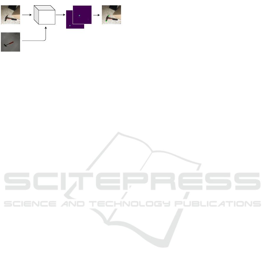
method presented in this paper is shown in Figure 1

This paper proposes a Fully Convolutional Neural

Network that generates heatmaps indicating the prob-

ability that a certain landmark is at the speciﬁed loca-

tion. The novel Intermediate Heatmap Model (IHM)

combines a feature detection network with upsam-

pling layers. Intermediate supervision is implemented

by generating output at multiple levels to boost the

Vanherle, B., Put, J., Michiels, N. and Van Reeth, F.

Real-time Detection of 2D Tool Landmarks with Synthetic Training Data.

DOI: 10.5220/0010689900003061

In Proceedings of the 2nd International Conference on Robotics, Computer Vision and Intelligent Systems (ROBOVIS 2021), pages 40-47

ISBN: 978-989-758-537-1

Real Images

Generated

Images

Training

Inference

Neural Network Heatmaps Keypoint Locations

Figure 1: An overview of the proposed method for keypoint

localization.

learning of higher level features. To prove the usabil-

ity of this method, it is compared to two existing key-

point detection methods on a custom tool dataset. The

method is also validated on the Pascal3D (Xiang et al.,

2014) dataset. Our main contributions are:

• A method for quickly generating images that are

suitable for deep learning, along with appropriate

labels.

• A Deep Learning architecture for keypoint detec-

tion that achieves good performance when trained

on synthetic images.

2 RELATED WORK

In classic computer vision, keypoint detection is

usually done using feature descriptors such as

SIFT (Lowe, 2004) or SURF (Bay et al., 2006). These

methods focus on local features and fail to consider

the global context of the image, hence why they do

not generalize well to unseen data and fail under vari-

ations of pose, lighting and texture.

In more recent works there has been a shift to-

wards Deep Learning to avoid these issues. Early

works, such as DeepPose (Toshev and Szegedy,

2014), would use a CNN to detect image features, fol-

lowed by fully connected layers that directly regress

the (x, y) coordinates of the keypoints. These meth-

ods had low accuracy, which lead to the creation of

networks that regress heatmaps for each keypoint.

Keypoint locations are computed from the maxima

of these heatmaps. This method has been used for

6DoF Pose Estimation (Pavlakos et al., 2017), Object

Detection (Law and Deng, 2020) and mainly for Hu-

man Pose Estimation (Wei et al., 2016; Newell et al.,

2016; Xiao et al., 2018). These methods are eas-

ier to train, but have difﬁculties detecting keypoints

when objects are occluded or truncated. For this rea-

son Pixelwise-Voting network (Peng et al., 2019) was

introduced. This type of network learns, for each key-

point, to generate unit vectors at each pixel pointing

to that keypoint. Those unit vectors are then used to

vote for keypoint locations using RANSAC (Fischler

and Bolles, 1981). This forces the network to focus

on local features and spatial relations between object

parts, and allows it to infer the position of invisible

parts.

The method proposed in this paper falls under the

category of heatmap generating models. Although

the pixel-wise voting method can handle occlusions

better, the RANSAC voting adds extra computational

complexity at runtime which is to be avoided in a real-

time system. Existing heatmap models often have

fast inference times, but rely on real images with an-

notations as training data. Our method removes this

need by offering a data generation method and a deep

learning model that performs well, when trained on

synthetic images.

3 TRAINING DATA

3.1 Image Generation

A key challenge of using a data-driven approach is

data collection. Training a model for a real-time 2D

landmark detection requires the collection of sufﬁ-

cient training data with a broad range of variations

for each physical tool at hand. Such training datasets

are not easily available and building new ones re-

quires access to large amounts of representative exist-

ing image data. Additionally, manual labor for iden-

tifying the ground truth 2D landmarks is required,

which is cumbersome and introduces human error to

the dataset. Furthermore, this approach does not gen-

eralize well when new types of physical tools are in-

troduced.

To avoid the time consuming process of taking

and manually labeling thousands of photos of tools,

we propose a synthetic data generation tool to eas-

ily generate training sets of newly introduced tools.

Synthetic data generation is often done by using a

Cut and Paste strategy (Dwibedi et al., 2017; Ghiasi

et al., 2020). This entails cutting the foreground ob-

jects from a limited set of images and pasting these at

randomized locations on random backgrounds. This

method lends itself well to Object Detection and Seg-

mentation problems, as those labels can be directly

inferred from the image composition. Although this

method can quickly generate large datasets, the im-

ages produced are often not realistic and lack varia-

tion in appearance, as the foreground objects are typi-

cally sourced from a very limited set. This could have

a negative impact on the accuracy of the keypoint lo-

calization. We therefore propose a tool that can ren-

der a set of images by constructing fully random 3D

Real-time Detection of 2D Tool Landmarks with Synthetic Training Data

scenes with the desired objects in them.

This tool will allow for more intricate appearance

and 3D variations than the classic data augmentation

techniques such as noise and translation. Examples

of more representative variations are 3D physical tool

rotations, translations, camera pose, occlusions, shad-

ows, lighting conditions, etc. Furthermore, we aim to

generate images as photorealistically as possible, as

this has been shown to improve performance on other

deep learning tasks (Hoda

n et al., 2019). To achieve

this, we have exploited the real-time raytracing capa-

bilities of recent NVidia RTX hardware.

To be able to create a scene with the desired object

in it, a 3D model of the object is needed. These can be

acquired by either performing a 3D scan or by manu-

ally modeling the object in CAD software. Both these

options are time consuming and can introduce errors.

We argue that this can be avoided by using a set of 3D

models of variations on the object, as opposed to one

exact model of the object. These variations can differ

in shape or texture, as long as they portray the same

type of object. By training a neural network on a set

of tools that all sufﬁciently vary in appearance, the

network will generalize to unseen tools of the same

kind. This allows us to simply source our 3D models

from the internet, for example.

The main input of this tool is a set of textured 3D

meshes of the physical tools. The tool will automat-

ically generate a wide range of variations based on

these models. The following parameters are random-

ized:

• Object position

• Object rotation

• Environment

• Lighting

Each random sample will be rendered with a path

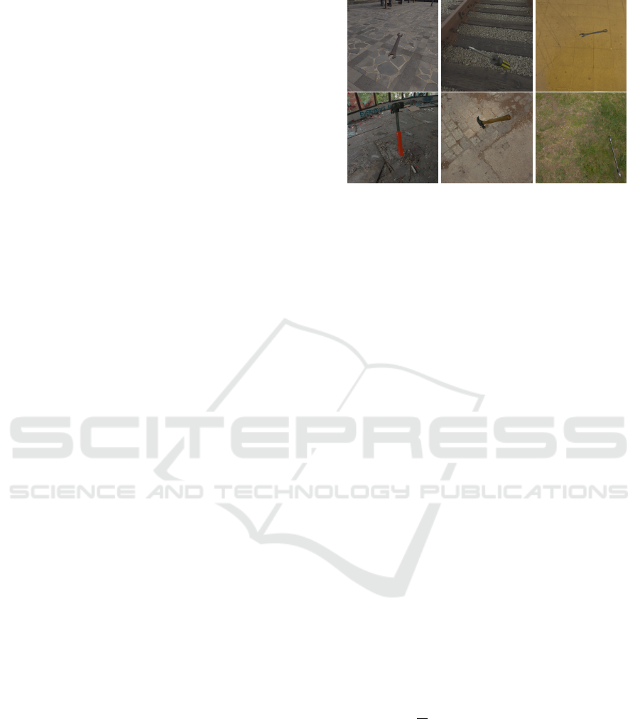
tracer to create a photo-realistic image. Figure 2

shows different examples of randomly generated syn-

thetic image data. An advantage of using such a syn-

thetic data generator is that we can export any kind of

additional labeled metadata as well. Here, the ground

truth 2D positions of the landmarks are exported to-

gether with the rendered images. This results in an

automatic approach for generating large amounts of

data needed for training deep learning networks such

as the one presented in Section 4.1. The use of path

tracing ensures a sufﬁcient amount of visual realism.

To further increase the size of the dataset and to

add occlusions, a copy of each image is added to

the dataset with a random object pasted in front of

it, or with the background switched out for a random

one. Foregrounds and backgrounds are added to the

image using a random blending method to avoid the

Figure 2: Synthetically generated images of tools.

network focusing on pixel artifacts, as described by

(Dwibedi et al., 2017). Blending was either done by

alpha blending, Poisson blending (P

erez et al., 2003)

or Laplacian pyramid blending (Burt and Adelson,

1983).

3.2 Heatmaps

In the proposed method, a Convolutional Neural Net-

work is used to interpret the image. This creates a

feature map. The locations of the keypoints need to

then be extracted from this feature map. This could

be done by ﬂattening the features and using one or

more fully connected layers to transform that vector

into the coordinate values of the keypoints. The ﬂat-

tening operation obfuscates the spatial information,

and the fully connected layers, unlike convolutional

layers, are not spatially invariant. This adds learning

complexity that leads to lower accuracy. A better ap-

proach is to use a fully convolutional neural network

that generates a set of heatmaps, as opposed to nu-

merical coordinates. A heatmap is generated for each

keypoint and contains, for each pixel, the probabil-

ity that the keypoint is at that location. Such a set of

heatmaps can be derived from the feature map by us-

ing convolutions, which uses the spatial information

more efﬁciently.

To construct the training data for an image a

heatmap is generated for each keypoint. A heatmap is

created by placing a two-dimensional Gaussian ker-

nel, with σ =

· width, centered at the 2D image lo-

cation of the keypoint. A smaller value for σ would

make it difﬁcult for the network to learn, whereas

a higher value would decrease localization accuracy.

Using this method, the value of the heatmap is 1.0 at

the keypoint location, with values tapering off further

away from the keypoint. An alternative to this is to

only make the correct pixel 1.0, but this is difﬁcult to

learn due to the overwhelming amount of zero values.

Assigning 1.0 to a larger area around the ground truth

pixel would solve this, but this would make it impos-

ROBOVIS 2021 - 2nd International Conference on Robotics, Computer Vision and Intelligent Systems

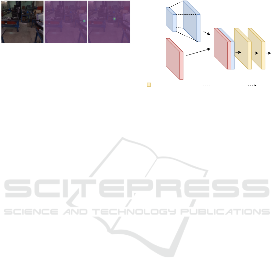
Figure 3: Synthetically generated image of a combination

wrench and the two heatmaps that the neural network will

try to predict.

sible to retrieve the exact pixel location. A Gaussian

kernel is therefore ideal in this scenario. Figure 3

shows the two Gaussian heatmaps generated for the

two keypoints of a combination wrench. When key-

points are very similar, as is the case for the two ends

of an open ended wrench, the heatmaps are added to-

gether into one heatmap. This removes ambiguity,

making learning easier.

During inference, the maximum of each heatmap

is computed to ﬁnd the pixel location of that keypoint.

When the heatmaps are compressed into one heatmap,

for the case of similar keypoints, local maxima are

then used as keypoint locations instead of the global

maximum. The value of the maximum pixel can be

interpreted as the conﬁdence of the prediction, which

can be used to threshold less certain predictions.

4 METHOD

4.1 Network Architecture

A Fully Convolutional Neural Network is trained to

generate these heatmaps. To be able to detect features

from real images while being trained on synthetic

images, a pre-trained feature detector is used. Dur-

ing training the feature detector’s layers are frozen,

as proposed by (Hinterstoisser et al., 2017). This is

done so that it cannot learn low-level features from

the synthetic data as these would not match the fea-

tures from real images. This has the additional bene-

ﬁt of decreasing the number of required training sam-

ples and time. ResNet50 (He et al., 2015) is used as

it offers good performance due to its relatively small

size, while still achieving good accuracy. The net-

work is pretrained on ImageNet (Deng et al., 2009).

This is the transfer learning aspect of our approach,

as knowledge learned from real images is transferred

the synthetic domain.

Using consecutive Residual Blocks, ResNet

down-samples the (224, 224, 3) input image to a

(7, 7, 2048) feature map. The resulting feature map

is up-sampled ﬁve times to generate a feature map of

Skip

Connection

Feature

Map

3x3 Conv + BN + ReLU DropoutNN upsampling

Figure 4: Illustration of the upsampling block.

size (224, 224, f ) with f the number of ﬁlters used.

Upsampling happens by using nearest neighbour in-

terpolation to double the width and height of the fea-

ture map. Skip connections are used to recover the

spatial information that was lost during downsam-

pling to increase the accuracy of the ﬁnal heatmaps.

This is done by concatenating the output of the ﬁnal

activation layer from the corresponding size from the

ResNet to the up-sampled feature map. This is fol-

lowed by two convolutional blocks, consisting of a

2D convolution with kernel size 3, Batch Normaliza-

tion (Ioffe and Szegedy, 2015), a Leaky ReLU and a

Dropout (Srivastava et al., 2014) layer with a rate of

0.2. An illustration of the upsampling block is shown

in Figure 4. The lowest level convolutions use 256 ﬁl-

ters, this amount is divided by two, each time the fea-

ture map is up-sampled. Finally, a convolution with

kernel size one, N ﬁlters and a sigmoid activation is

applied to generate the ﬁnal heatmaps. N is the de-

sired number of heatmaps.

When training neural networks on synthetic data it

is desirable that the network uses high level features

when generating output as opposed to focusing on

lower level features. This is because higher level fea-

tures, such as shape, match between synthetic and real

images; whereas lower level features, such as texture,

can differ tremendously. In a classic FCN, output is

generated at the ﬁnal upsampling step. This means

that, when using skip connections, output is created

from the upsampled feature map combined with the

lowest level features from the feature detector net-

work. This could lead to the network lazily focus-

ing on these lower level features, which we are trying

to avoid. Intermediate supervision is used to force

the network to learn good features that assist in local-

izing the keypoints, at each level of the upsampling

chain. This is implemented by generating a heatmap

after each upsampling block and using each heatmap

in the loss function. So as opposed to outputting one

Real-time Detection of 2D Tool Landmarks with Synthetic Training Data

7x7 conv stride 2

3x3 conv + max pool

7x714x1428x2856x56112x112

downsampling ResBlock

ResBlock

upsampling block

1x1 conv + sigmoid

input

image

224x224

14x14

heatmap

224x224

heatmap

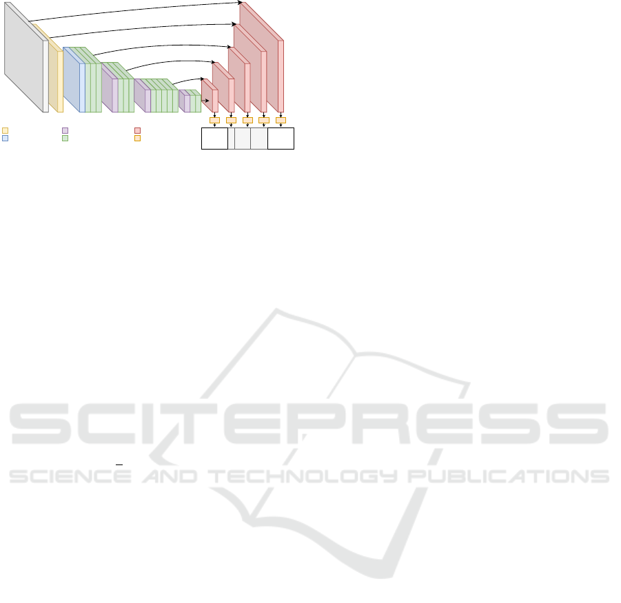
Figure 5: A full overview of the neural network used to

generate heatmaps.

heatmap, the network generates a set of progressively

larger heatmaps, starting at (14, 14) up to (224, 224).

By applying this type of supervision at each upsam-

pling level, the learning of high level features gets

boosted, while lower level features can also still be

used to generate the ﬁnal output. Although, poten-

tially less accurate, each of the intermediate heatmaps

can be used to localize keypoints. A full overview of

the neural network is given in Figure 5.

4.2 Training

The loss function is the sum of the Mean Squared Er-

ror between the heatmap generated at each level and

their corresponding ground truth.

L =

∑

(

∑

( f

) −Y

k,n

)) (1)

Here f

is the output of the k-th upsampling block, X

the n-th image and Y

k,n

the ground truth heatmaps for

the n-th image, downscaled to the size of the k-th out-

put. Training is done using the ADAM (Kingma and

Ba, 2017) optimizer with a learning rate of 1.5e

−5

The learning rate is scaled by 0.1 if the validation loss

has not improved for 10 epochs. A batch size of 16

is used with a maximum of 200 epochs. The network

stops training after showing no improvement for 20

epochs. The loss on the validation set is measured at

each epoch and the model with the lowest validation

error is kept. To improve robustness and generaliza-

tion towards real life images, a wide range of data

augmentation techniques are applied to the images.

These include afﬁne transformations, blurring, adding

and multiplying, perspective transformations and ad-

ditive Gaussian noise. When transformations are ap-

plied, the heatmaps are adapted correspondingly.

5 RESULTS

The proposed method is ﬁrst validated on a dataset

of tool images created speciﬁcally for this paper. To

show this method generalizes well to other domains

and to compare the results of this paper to an estab-

lished benchmark, the method is also validated on the

Pascal3D dataset (Xiang et al., 2014). Our approach

has been compared to two other methods for keypoint

detection: Stacked Hourglass Networks (SH) (Newell

et al., 2016; yuanyuanli85, 2018) with two stacks and

Simple Baselines (SB) (Xiao et al., 2018). The for-

mer is chosen as it is used often, achieves great accu-

racy and also employs a form of intermediate super-

vision. Since this method does not use transfer learn-

ing, the latter is also selected for validation, as trans-

fer learning might give an advantage when training

on synthetic data. A comparison is also made with a

trimmed version of our IHM, that generates heatmaps

of size (56, 56) (IHM

), and with a version of our

model that was trained without intermediate supervi-

sion (HM).

The Percentage of Correct Keypoints (PCK) metric is

used to validate performance. A keypoint is consid-

ered to be correct when its distance from the ground

truth is below a certain fraction of the largest side of

the objects bounding box: α · max(w, h), with α usu-

ally at 0.1.

In the experiments described below, we train a sep-

arate neural network for each object, as opposed to

one network that can predict the keypoints of each

object. The beneﬁt of this approach is that a smaller

network is required for each tool, leading to better

execution times. For this it is assumed that the sys-

tem knows which tools keypoints need to be found,

as executing the network for each tool would have the

opposite effect on the total execution time. Another

beneﬁt of this approach is that new objects can eas-

ily be introduced into the system by simply training a

new network for only that tool. Although training one

large network for all objects could also have bene-

ﬁts. Potentially, less training images per object could

be needed, as feature learning would be shared, and

features could be learned from each object. Addition-

ally this approach could decrease sensitivity to false

positives, as the network sees different types of tools

during training.

5.1 Tool Dataset

To validate our work, a dataset of images has been

created for four different tools. Of each tool 50 pho-

tographs are created with a mobile phone camera.

Photos are taken with a wide range of backgrounds,

ROBOVIS 2021 - 2nd International Conference on Robotics, Computer Vision and Intelligent Systems

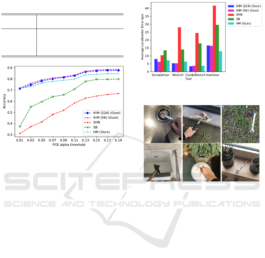
Table 1: Comparison of the IHM, HM, SH and SB methods

on the Tool Dataset (PCK

α=0.1

Model IHM

224

IHM

HM SHN SB

(Ours) (Ours) (Ours)

Screwdriver 82.0 82.0 78.0 46.0 74.0

Wrench 88.9 88.9 86.1 66.7 67.6

C. Wrench 84.9 84.9 82.6 55.8 68.6

Hammer 72.9 74.0 68.8 45.8 63.5

Figure 6: PCK values for the ﬁve examined models for

varying thresholds.

lighting conditions, camera rotations and positions.

The tools are often truncated or partially occluded by

hands or other objects. The images are manually an-

notated with keypoint locations. For each tool six to

ten different 3D models with textures were collected

from the internet. These models were used to gener-

ate a dataset of 10.000 training images as described

in Section 3. For each tool, the ﬁve different models

were trained on that dataset.

For each model the PCK value was computed on the

validation dataset of real images, the results are dis-

played in Table 1. For each of the four tools, the In-

termediate Heatmap Model outperforms the Simple

Baseline and Stacked Hourglass models. The latter

is outperformed by a large margin, highlighting the

importance of transfer learning when using synthetic

training data. Also the model without intermediate

supervision is outperformed for each tool, showing

the importance of this learning method. To further

examine the accuracy, the performance of the mod-

els is measured for differing α values for the PCK.

The results, shown in Figure 6, indicate that IHM has

a way better localization error, as it manages to still

achieve a good PCK score at a very low α value com-

pared to the other models. Remarkably, the IHM

model with two less upsampling layers performs as

well as, or better than the full IHM model. To fur-

ther examine this, the distance between the keypoints

that were correctly predicted with α = 0.1 and the ac-

Figure 7: Average localization error for correctly predicted

keypoints at α = 0.1. The images are of size (224, 224).

Figure 8: Six examples from the tool dataset. Predictions

made by the IHM

model are indicated by the dots. Cor-

rectly predicted images were chosen.

tual ground truth is computed. These results per class

are shown in Figure 7. The IHM

224

model has an

average localization error of 8.4px for correctly pre-

dicted keypoints, whereas the IHM

model has an er-

ror of 7.9px. The SHN and SB methods have an error

of 25.2px and 18.8px respectively. This shows that

the ﬁnal upsampling layers, that utilize the low-level

features from the feature detector, offer no beneﬁt to

the ﬁnal accuracy. This indicates the importance of

high level features when training on synthetic data.

Some correct predictions made by the best perform-

ing model IHM

are shown in Figure 8.

5.1.1 Performance

The time needed to process an image is 0.04 sec-

onds on average for all our models, this equates to

25 frames per second. This time includes all post-

processing done to ﬁnd the keypoint locations from

the generated heatmaps. This time was measured

on a machine with an NVidia GeFore RTX 2080 su-

per. The other models performed within comparable

times.

Real-time Detection of 2D Tool Landmarks with Synthetic Training Data

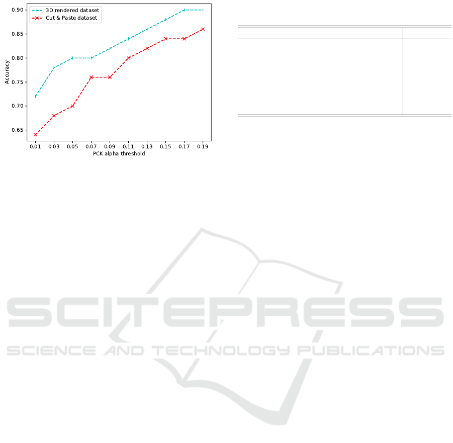
Figure 9: PCK values for varying α thresholds of the IHM

model trained on the Cut and Paste dataset compared to our

3D dataset.

5.1.2 Cut and Paste vs. 3D Generated Training

Data

To show the importance of using 3D generated train-

ing images for keypoint localization, as opposed to

cut and paste 2D images, an extra experiment is con-

ducted, comparing the two methods. For this ex-

periment the focus is on the screwdriver class. An

extra set of images with ground truth annotations is

created according to the method of (Dwibedi et al.,

2017). Images of ten different screwdrivers were col-

lected from the internet and their backgrounds were

removed. They were added to random background

images with a random rotation, translation and scale

using a random blending mode, as described in Sec-

tion 3 and (Dwibedi et al., 2017). This process was

repeated to generate 10.000 images. This dataset was

then used to train a version of the IHM model. This

model is compared to the model trained on the 3D

generated data. This comparison for a varying range

of α values can be seen in Figure 10. The model

trained on 3D data clearly outperforms the model

trained on the Cut and Paste generated images. This

shows that the extra variation that 3D generated data

brings has a clear beneﬁt for the task of keypoint lo-

calization.

5.2 Pascal3D Dataset

As no established dataset or benchmark exists for this

speciﬁc problem, the proposed method is also vali-

dated on the Pascal3D dataset. Since the results from

the previous section already show that our method

generalizes to real images when trained on synthetic

ones, the focus is now on purely validating the task of

keypoint detection. Hence, for the Pascal3D dataset,

we train on the real images provided by the dataset

Table 2: Comparison of selected methods on the PAS-

CAL3D Dataset.

Method PCK

α=0.1

IHM

(Ours) 74.2

HM (Ours) 76.7

Pavlakos et al. (Pavlakos et al., 2017) 82.5

Zhou et al. (Zhou et al., 2018) 78.6

Tulsiani et al. (Tulsiani and Malik, 2014) 68.8

Long et al. (Long et al., 2014) 48.5

Simple Baseline (Xiao et al., 2018) 42.7

and not synthetic ones generated by our method. For

each of the classes in the dataset a separate model is

trained to detect the keypoints speciﬁed in the dataset.

A separate validation set is withheld from training and

used to compute the PCK values.

The results of our models are compared to those of

a number of existing methods. This is shown in Ta-

ble 2. The PCK values are taken from the methods

respective papers. For the (Pavlakos et al., 2017)

method, the PCK value was computed by (Zhou et al.,

2018). Our IHM

model achieves an accuracy of

74.2 whereas our HM model achieves 76.7 PCK. In-

terestingly the model with intermediate supervision

performs worse than the model without. This indi-

cates that intermediate heatmap generation improves

accuracy when training on synthetic data, but is not

of useful when training is done using real data. Our

method performs well for most classes, achieving

+90% accuracy for the bus and car classes, but the

score is lowered signiﬁcantly by bad performance on

the dining table and train classes. These results show

that, although not achieving state-of-the-art, the pro-

posed method still achieves decent performance when

applied to a different domain. The focus of this paper

is to detect tool keypoints in real-time when trained

on synthetic data, so scoring only 5.8 points below

SoA on a different task is reasonable.

6 CONCLUSION

In this paper a method for real-time tool keypoint

localization was proposed, along with a method for

synthetic data generation. Models were successfully

trained to detect the landmarks of four different tools

in real images, proving the usability of the proposed

data generator tool. It was shown that the method out-

performs existing methods at the task by predicting

the keypoints with a higher accuracy. Additionally

the importance of intermediate supervision when us-

ing synthetic data was shown, as a copy of our model

that does not use this scheme performs worse on syn-

thetic data. Furthermore, we have shown that an exact

ROBOVIS 2021 - 2nd International Conference on Robotics, Computer Vision and Intelligent Systems

3D model of an object is not necessary when generat-

ing synthetic training images, as long as a set of vary-

ing 3D models are used. Validation on the Pascal3D

dataset has shown that this method also generalizes to

domains other than tools.

ACKNOWLEDGEMENTS

This study was supported by the Special Research

Fund (BOF) of Hasselt University. The mandate ID

is BOF20OWB24. Research was done in alignment

with Flanders Make’s PILS and FAMAR projects.

REFERENCES

Bay, H., Tuytelaars, T., and Van Gool, L. (2006). Surf:

Speeded up robust features. In Leonardis, A., Bischof,

H., and Pinz, A., editors, Computer Vision – ECCV

2006, pages 404–417, Berlin, Heidelberg. Springer

Berlin Heidelberg.

Burt, P. J. and Adelson, E. H. (1983). A multiresolution

spline with application to image mosaics. ACM Trans.

Graph., 2(4):217–236.

Deng, J., Dong, W., Socher, R., Li, L.-J., Li, K., and Fei-

Fei, L. (2009). Imagenet: A large-scale hierarchical

image database. In 2009 IEEE conference on com-

puter vision and pattern recognition, pages 248–255.

Ieee.

Dwibedi, D., Misra, I., and Hebert, M. (2017). Cut, paste

and learn: Surprisingly easy synthesis for instance de-

tection. pages 1310–1319.

Fischler, M. A. and Bolles, R. C. (1981). Random sample

consensus: A paradigm for model ﬁtting with appli-

cations to image analysis and automated cartography.

Commun. ACM, 24(6):381–395.

Ghiasi, G., Cui, Y., Srinivas, A., Qian, R., Lin, T.-Y., Cubuk,

E. D., Le, Q. V., and Zoph, B. (2020). Simple copy-

paste is a strong data augmentation method for in-

stance segmentation.

He, K., Zhang, X., Ren, S., and Sun, J. (2015). Deep resid-

ual learning for image recognition.

Hinterstoisser, S., Lepetit, V., Wohlhart, P., and Kono-

lige, K. (2017). On pre-trained image features

and synthetic images for deep learning. CoRR,

abs/1710.10710.

Hoda

n, T., Vineet, V., Gal, R., Shalev, E., Hanzelka, J.,

Connell, T., Urbina, P., Sinha, S. N., and Guenter, B.

(2019). Photorealistic image synthesis for object in-

stance detection. In 2019 IEEE International Confer-

ence on Image Processing (ICIP), pages 66–70.

Ioffe, S. and Szegedy, C. (2015). Batch normalization: Ac-

celerating deep network training by reducing internal

covariate shift. CoRR, abs/1502.03167.

Kingma, D. P. and Ba, J. (2017). Adam: A method for

stochastic optimization.

Law, H. and Deng, J. (2020). Cornernet: Detecting objects

as paired keypoints. International Journal of Com-

puter Vision, 128.

Long, J., Zhang, N., and Darrell, T. (2014). Do convnets

learn correspondence? CoRR, abs/1411.1091.

Lowe, D. (2004). Distinctive image features from scale-

invariant keypoints. International Journal of Com-

puter Vision, 60:91–.

Newell, A., Yang, K., and Deng, J. (2016). Stacked hour-

glass networks for human pose estimation. In Leibe,

B., Matas, J., Sebe, N., and Welling, M., editors, Com-

puter Vision – ECCV 2016, pages 483–499, Cham.

Springer International Publishing.

Pavlakos, G., Zhou, X., Chan, A., Derpanis, K. G., and

Daniilidis, K. (2017). 6-dof object pose from semantic

keypoints. In 2017 IEEE International Conference on

Robotics and Automation (ICRA), pages 2011–2018.

Peng, S., Liu, Y., Huang, Q., Zhou, X., and Bao, H. (2019).

Pvnet: Pixel-wise voting network for 6dof pose esti-

mation. pages 4556–4565.

erez, P., Gangnet, M., and Blake, A. (2003). Poisson im-

age editing. ACM Trans. Graph., 22(3):313–318.

Srivastava, N., Hinton, G., Krizhevsky, A., Sutskever, I.,

and Salakhutdinov, R. (2014). Dropout: A simple way

to prevent neural networks from overﬁtting. Journal

of Machine Learning Research, 15(56):1929–1958.

Toshev, A. and Szegedy, C. (2014). Deeppose: Human pose

estimation via deep neural networks. In 2014 IEEE

Conference on Computer Vision and Pattern Recogni-

tion, pages 1653–1660.

Tulsiani, S. and Malik, J. (2014). Viewpoints and keypoints.

CoRR, abs/1411.6067.

Wei, S., Ramakrishna, V., Kanade, T., and Sheikh, Y.

(2016). Convolutional pose machines. In 2016 IEEE

Conference on Computer Vision and Pattern Recogni-

tion (CVPR), pages 4724–4732.

Xiang, Y., Mottaghi, R., and Savarese, S. (2014). Beyond

pascal: A benchmark for 3d object detection in the

wild. In IEEE Winter Conference on Applications of

Computer Vision (WACV).

Xiao, B., Wu, H., and Wei, Y. (2018). Simple baselines

for human pose estimation and tracking. In Ferrari,

V., Hebert, M., Sminchisescu, C., and Weiss, Y., edi-

tors, Computer Vision – ECCV 2018, pages 472–487,

Cham. Springer International Publishing.

yuanyuanli85 (2018). Stacked

hourglass network keras.

https://github.com/yuanyuanli85/Stacked Hourglass

Network Keras.

Zhou, X., Karpur, A., Luo, L., and Huang, Q. (2018).

Starmap for category-agnostic keypoint and viewpoint

estimation. CoRR, abs/1803.09331.

Real-time Detection of 2D Tool Landmarks with Synthetic Training Data