Efﬁcacy of Statistical Formulations on Acoustic Emission Signals for Tool

Wear Predictions

Selvine G. Mathias

and Daniel Grossmann

Technische Hochschule Ingolstadt, Esplanade 10, 85049 Ingolstadt, Germany

Keywords:

Acoustic Emission, Tool Wear, Data Imputations, Statistical Approach.

Abstract:

Acoustic emission (AE) signals obtained during machining processes can be used to detect, locate and assess

ﬂaws in structures made of metal, concrete or composites. This paper aims to characterize AE signals using

derived parameters from raw signatures along with statistical feature extractions to correlate with tool wear

readings. Missing tool wear values are imputed using domain knowledge rules and compared to AE signals

using machine learning models. The amount of effect on tool wear is formulated using Bayesian Inferences

on derived parameters such as areas under the raw signal curve in addition to comparisons with the supervised

models for predictions. Using the constructed models and formulation, the presented study also includes a

trace-back pseudo-algorithm for determining the stage in process where tool wear values begin to approach

the wear limits.

1 INTRODUCTION

A material under stress releases elastic waves from

localized deformation sources such as cracks, dislo-

cations, etc. which are termed as Acoustic Emis-

sions. Sources generating AE in different materials

are unique. For examples, in metals, primary macro-

scopic sources are crack jumps, processes related to

plastic deformation development and fracturing and

de-bonding of inclusions. Quantitative and qualita-

tive characteristics of acoustic emission waves, gener-

ated by sources of different nature depend directly on

material properties and environmental factors (Grosse

and Ohtsu, 2008). Hence, with advanced technologies

available to capture and process AE signals in modern

applications, the use of AE in detection and analysis

of ﬂaws, cracks, corrosion and abnormal conditions in

metals has advanced steadily along the lines of statis-

tical analysis, machine learning and data understand-

ing (Al-Jumaili et al., 2016).

Conventional methods like statistical and wavelet

analyses are still available and in some cases, the pre-

ferred modes of analyzing AE signatures which is ev-

ident in (Singh et al., 2012) where piezoelectric sen-

sors were used to identify micro and macro-cracks

and their temporal advancement in snow to detect

avalanches. In general, with the objectives set in de-

https://orcid.org/0000-0002-6549-0763

tecting sources of ﬂaws in metals during processes,

the application of feature extractions in AE signals is

an area of research that are conducted based on the

kind of problem at hand, for example, detection of

leaks, friction, knocks, chemical reactions, changes of

size of magnetic domains, apart from deformationand

fracture development in structures. Hence, the devel-

opment of AE technologies relies on understanding

the physical nature of acoustic emission in different

materials. To achieve this goal, determination of the

interconnections between characteristics of acoustic

emission and sources that generated it, is of utmost

importance. However, establishing such relations for

different materials and structures is a real scientiﬁc

and technological challenge. The tasks of reaching

the correct machining conditions, constructing instru-

mentation and setups (Chiementin et al., 2010), build-

ing data acquisition modules along with predictive

networks (Suwansin and Phasukkit, 2021) undeniably

contribute variations to AE readings along with the in-

tended capture of the source emissions. From a data

mining point of view, a primary problem of analysing

AE signals is to be able to derive sustainable param-

eters from the raw data for comparisons with targets

such as crack depths or tool wear amounts or machin-

ing temperatures. Since material cutting and defor-

mations effect a certain change in the tools used, a

variety of studies focus on establishing links between

material changes using AE sensors and damages or

108

Mathias, S. and Grossmann, D.

Efﬁcacy of Statistical Formulations on Acoustic Emission Signals for Tool Wear Predictions.

DOI: 10.5220/0010676400003062

In Proceedings of the 2nd International Conference on Innovative Intelligent Industrial Production and Logistics (IN4PL 2021), pages 108-115

ISBN: 978-989-758-535-7

wears incurred by the tools (Bhuiyan et al., 2016).

This study aims to develop models between mul-

tiple features from the AE signals such as areas un-

der curves of the signal, categorical features fed into

the process and progressive tool wear observed dur-

ing the runs. Sections 2 and 3 present the associated

works and the developed scheme for comparing AE

data with tool wear values. Sections 4 and 5 discuss

the results observed from the models with possible in-

tegration scenario in industrial applications and con-

cluding remarks.

2 ASSOCIATED LITERATURE

Notable literature using acoustic emissions in their

study present mainly two kinds of analysis: conven-

tional studies using signal analysis and machine learn-

ing techniques. The conventional methods comprise

of extracting statistical data indicators such as Root-

Mean-Square values, kurtosis, signal envelope, etc.

Early studies using statistical relations based on AE

comprised of detecting correlations between AE and

physical characteristics of materials such as (Carpen-

ter and Zhu, 1991), (Pearson et al., 2017), where cor-

relations were observed between AE signals and frac-

ture toughness of cast iron under compression tests.

In (Usgame et al., 2013), the authors present a com-

parison of time based fault indicators such as peak

value, RMS, ring-down counts and kurtosis to detect

faults in tapered roller bearings. In recent decades,

structural health monitoring (SHM) has become an

inclusive concept of developing methods for prognos-

tic and diagnostic monitoring of engineering builds

based on materials (Khan, 2018), for example inspec-

tions of bolted joints (Du et al., 2018), metal pressure

vessels, pipes, concrete bridges, rotating machinery,

cutting tools, etc. with the help of material studies.

Some specialized statistical approaches are also de-

veloped in the context of obtaining signiﬁcance of sig-

nal unbalances in machine equipment. This was used

in (Niknam et al., 2013) where a Zero-Inﬂated Pois-

son (ZIP) regression model was developed to han-

dle over-dispersion and zeros of the counting data

from bearings along with Generalized Linear Models

(GLM) which were used to perform categorical data

analysis.

With modern data based learning techniques such

as machine learning (ML) and deep learning (DL), the

studies involving AE data has expanded to include lo-

calization and fault detection problems using AE sig-

natures on a large scale. In (Suwansin and Phasukkit,

2021), the authors constructed a specialized neural

network with a majorization-minimization cost func-

tion optimization to predict cracks in welding joints

of steel rail under a load using a single AE sensor.

The results from the study were also compared with

actual results obtained directly from Phased Array Ul-

trasonic Testing (PAUT) and they showed that the

accuracy scores of the proposed AE based scheme

reached 77.33%. Image based deep learning was im-

plemented in (Mokhtari et al., 2020) on AE image

data to localize crack sources and defects. The com-

putational expenses were also huge as compared to

traditional studies. An array of AE sensors with SVM

techniques have also been used for analysis in (del Val

et al., 2020).

In (Bhuiyan et al., 2016), the progressivetool wear

in turning process was studied using continuous mon-

itoring of the amplitudes of AE signals obtained from

piezoelectric sensors placed on the tool holder. The

continuous type signals were observed for different

feed rates and depth of cuts factors to distinguish be-

tween observed signals with inherent noise from tool

holder setup along with chip formation and the pure

signals from only tool wear. The study determined

that the amplitude of AE signal increased with the

increase of tool wear and depth of cut i.e. with the

increased rate of material removal.

Even though each AE signal is a time series, the

complex dependency of tool wear on the different

phases of AE cannot be generalized using conven-

tional time series methods. Therefore, this study pro-

poses a work-in-progress prediction scheme that is

statistical model based, speciﬁcally Bayesian formula

based along with classiﬁcation and regression algo-

rithms to provide a complete monitoring process de-

void of dominant signal analysis. Temporal depen-

dencies are not considered, and with simple derived

parameters from the given pre-processed AE signals,

the authors here present a multi-modeling approach

on different cases of AE signals from the same milling

process based on different conditions. Classiﬁcations

to detect parameters fed before the process and regres-

sions to predict tool wear values for a given AE sig-

nals are implemented. The Bayesian model is used to

determine the pattern of tool wear degradation based

on derived parameters from the signals. These early

investigations are carried out on a single public data-

set to verify whether the models yield reasonable in-

ferences.

3 DATA MINING APPROACH

We begin this section with a description of the con-

sidered data followed by parameters deriving ap-

proaches. Further, machine learning models are built

Efﬁcacy of Statistical Formulations on Acoustic Emission Signals for Tool Wear Predictions

109

to assess the relationship between the different fea-

tures.

0 2000 4000 6000 8000

Tim e (m illiseconds)

0.10

0.15

0.20

0.25

0.30

Am plit ude (V)

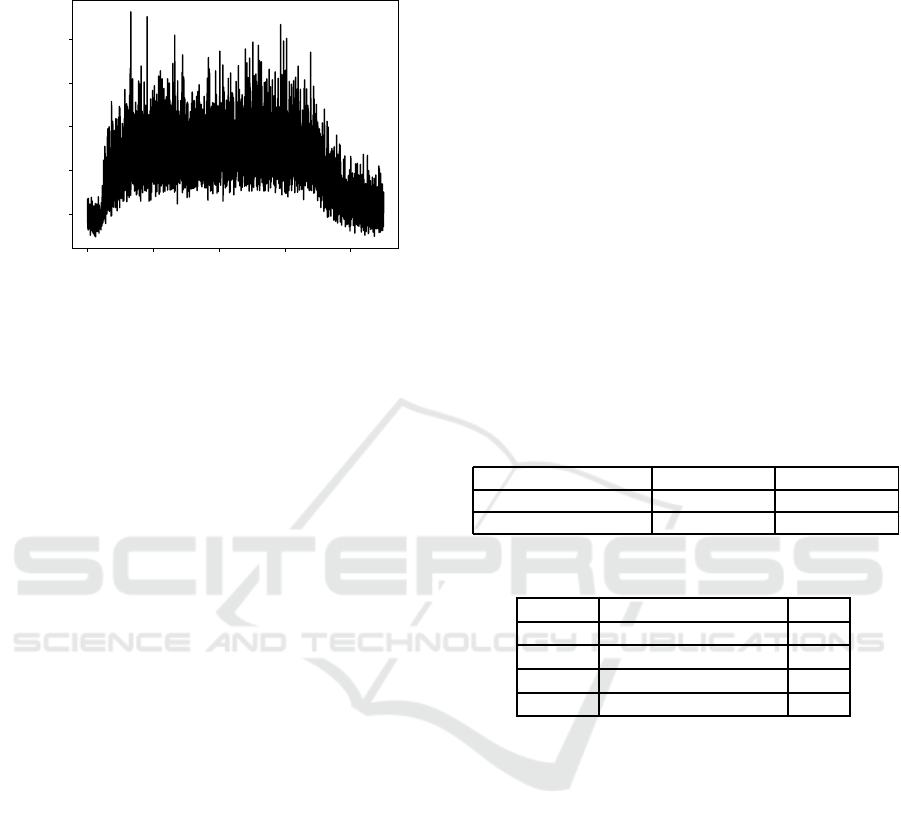
Figure 1: An Acoustic Emission Signal from Sensor

mounted on the Worktable.

3.1 Acoustic Dataset Description

The data used in this study is a collection of experi-

ments from runs on a milling machine under various

operating conditions (Agogino and Goebel, 2007). In

particular, tool wear was investigated in a regular cut

as well as entry cut and exit cut. Data was sampled

by three different types of sensors (acoustic emis-

sion sensor, vibration sensor, current sensor) and ac-

quired at several positions. This paper utilizes only

the acoustic raw signatures captured from the acous-

tic sensor model WD-925 (Physical Acoustic Group,

frequency range up to 2MHz) mounted on the table

of a Matsuura machining center MC-510V in the ex-

perimental set-up. The signals captured are ampli-

ﬁed, ﬁltered and fed through two RMS devices be-

fore they enter the computer for data acquisition. The

proposed analysis can also be conducted on the data

from the other AE sensor attached to the spindle and

hence, it is excluded from the study presented here.

The points are provided in raw format as amplitude

in volts against time in milliseconds. A typical AE

signature from the milling process where the sensor

was placed on the table next to the tool insert shaft

is shown in Figure 1. The collective data presents 16

cases with varying number of runs that was dependent

on the degree of ﬂank wear on the used tool measured

between runs at irregular intervals up to a wear limit

(and sometimes beyond). The readings were not al-

ways measured and at times when no measurements

were taken, no entry was made, presenting missing

values in the data. Hence, imputing rules are deﬁned

in later sections. The imputation is done using self-

constructed rules, knowing the behavior of the pro-

cesses involved. A brief distribution of these 16 cases

is presented in Table 1b with different parameters of

processes such as Depth of Cut (DOC), Feed and Ma-

terial. These factors form the external categorical fea-

tures used in training data. The tool wear recorded in

this process is the ﬂank wear that occurs due to fric-

tion of the tool on the work-piece.

The columns corresponding to an AE signature in

every case are run, Flank Wear, time, DOC, feed, and

material. We denote the variable Flank Wear in this

study with TW, denoting Tool Wear. Each captured

raw signature corresponds to one of the runs (some-

where in time), while it is noted that the captured sig-

nals are not uniformly recorded in time domain. So

the runs only tell the sequence of the consecutive AE

signals. The whole dataset of AE signals comprise of

165 observed samples over all the 16 cases and 2 ex-

periments with 9000 points for every AE signal. Fur-

ther description of the complete setup and experimen-

tation is provided in the read-me section given along

with the dataset.

Table 1: Data Description.

(a) Distribution of Cases across Materials and Experiments.

Experiment 1 Experiment 2

Material 1: Cast Iron 1,2,3,4 9,10,11,12

Material 2: Steel 5,6,7,8 13,14,15,16

(b) Distribution of Parameters across the Cases

Color Depth of Cut (DOC) Feed

Red 1.5 0.5

Purple 1.5 0.25

Blue 0.75 0.5

Orange 0.75 0.25

The selection of this data set is made on the basis

of availability of pre-processed AE signals for early

implementations, before validating this scheme and

using it on large scale industrial data-sets. Another

factor is the kind of unstructured data collected with

missing tool wear readings, presenting an opportunity

to apply a customized imputation scheme.

3.2 Usable and Derived Features from

the AE Data

A set of features that contribute to AE readings,

apart from the source generation and noise inheritance

along the transmission, are feeds, conditions and pa-

rameters that are set prior to the machining operation.

These factors are passive moderators to the variation

of emissions, in the sense that they are not actively

affecting tool wear as in the case of machine temper-

atures and sheer stress during the process.

IN4PL 2021 - 2nd International Conference on Innovative Intelligent Industrial Production and Logistics

110

0.00 0.25 0.50 0.75 1.00 1.25 1.50

Tool Wear (cm )

0.5

1.0

1.5

2.0

2.5

3.0

Area under AE Signal (Vs)

Correlat ion= 0.6543824644499396

0.00 0.25 0.50 0.75 1.00 1.25 1.50

Tool Wear (cm )

0.0

0.2

0.4

0.6

0.8

1.0

Peak Value of AE Signal (V)

Correlat ion= 0.5765157315046051

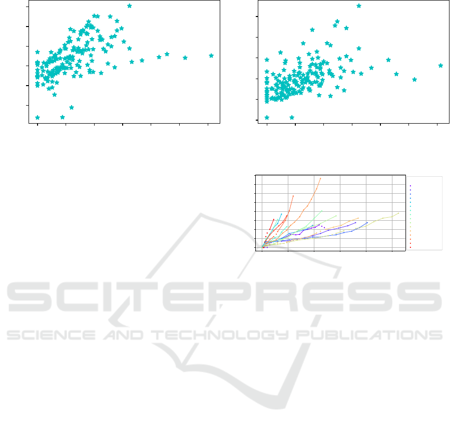
Figure 2: Distribution of Points with Correlation Values.

In addition to the available external features, to

develop links between AE data and tool wear, we ex-

tract single dimensional parameters from the signal

to compare with the target variable. The area under

the curve is extracted to correlate with tool wear us-

ing trapezoidal rule for integration. Another impor-

tant parameter for consideration is the peak ampli-

tude of the processed signal. Spearman’s correlation

coefﬁcient is calculated between the variables and is

presented in Figure 2. The values show that area is

highly correlated with the tool wear readings than the

peak values. Hence, we use the calculated areas in the

statistical model formulated in following sections.

3.2.1 Label Imputation Rules

Considering that every recorded AE signature may

not be accompanied with a tool wear reading, there

is a need to consider these samples in the training of

algorithms sensibly. To do it conventionally, a user

may be forced to either exclude these readings alto-

gether or ﬁll up the labels with either zero or the av-

erage of the readings. Instead in this case, we use the

given pattern of collected tool wear readings in a case

to ﬁll in the missing values. For every run, the miss-

ing value is ﬁlled by comparing with its previous or

next value.

The following algorithm was used to impute null

or missing tool wear readings TW(i) for an index i in

the data within the same case:

1. If TW(i) == Null with TW(i − 1)! = Null and

TW(i + 1)! = Null, then TW(i) = avg(TW(i −

1),TW(i+ 1))

2. If TW(i+ 1) == Null, then TW(i) = TW(i− 1)

3. If TW(i − 1) == Null, then TW(i) = TW(i +

1)/2

4. If i == 0, then TW(i) = 0

0 20 40 6 0 80 10 0

Machining Tim e (m s)

0. 0

0. 2

0. 4

0. 6

0. 8

1. 0

1. 2

1. 4

1. 6

Flank Wear wit h Im pu ted Point s (m m )

- Ob se r v ed

. Im p ut ed

Case 1 , Ma t erial 1

Case 2 , Ma t erial 1

Case 3 , Ma t erial 1

Case 4 , Ma t erial 1

Case 5 , Ma t erial 2

Case 6 , Ma t erial 2

Case 7 , Ma t erial 2

Case 8 , Ma t erial 2

Case 9 , Ma t erial 1

Case 1 0 , Mat eri al 1

Case 1 1 , Mat eri al 1

Case 1 2 , Mat eri al 1

Case 1 3 , Mat eri al 2

Case 1 4 , Mat eri al 2

Case 1 5 , Mat eri al 2

Case 1 6 , Mat eri al 2

Figure 3: Tool Wear Imputation using the Deﬁned Rules.

5. If i is last index, then TW(i) = TW(i− 1)

6. The above cases will eliminate TW(i − 1) ==

TW(i) == TW(i+ 1) == Null

Simplistically, a tool wear reading in sequence lies

between its previous and next values. For this study,

a missing tool wear value is ﬁlled by the average of

its previous and the next tool wear values. It assumes

its previous value if its next value is missing or half of

the next value if the previous value is missing. With

sequential application in each case, the algorithm will

eliminate those cases where both the next as well as

previous values are missing. The imputed tool wear

readings are shown in Figure 3.

3.3 Predictive Models

Considering the imputed tool wear readings as tar-

get, the entire AE data is trained with four regressors,

namely Ordinary Least Squares, i.e. Linear, Lasso,

Elastic Net and LassoLars. The choice of using the

complete data is made to enable the use of scalable

Big Data based algorithms when the emissions are

captured with a higher frequency rate and at more

intervals. Each of the regressors was trained with a

cross validation split of 70%-30%, apart from the un-

known test set. The regression values determine the

approximateamount of tool wear for that captured AE

Efﬁcacy of Statistical Formulations on Acoustic Emission Signals for Tool Wear Predictions

111

signal. Mean absolute error and mean squared error

are the metrics used to validate the models on the test

set.

Along with regression models, a supervised learn-

ing to yield classiﬁcations of the AE signatures is also

constructed. The predictions of tool wear readings

were done on case to case basis, since each case has

its own parametric features that affected the milling

process. Without considering the temporal effects on

the runs of each case, the attempt to learn the pre-

set external factors selected before the milling pro-

cess is made to identify relationships between the

captured AE signals and the concerned factor. The

three factors considered for individual classiﬁcation

are DOC, Feed and Material. The classiﬁcation mod-

els are trained on the entire raw signature data set with

the samples shufﬂed indiscriminately to learn the pat-

terns locally. The data is re-scaled before training

using a kernel transformation based on the means of

each case. The kernel product reduces the number of

columns to 16, one corresponding to each case. The

classiﬁers range from linear models such as logistic

regression to tree-based algorithms such as decision

tree and random forest. The linear and quadratic dis-

criminant analysis algorithms are used as well. Cross-

validation with a split of 70%-30% train-test data is

used to reduce overﬁtting in the models, as in the

case of the regression models, with a separate set of

the unknown test data. At this stage of investigation,

the authors have presented only the necessary mod-

els to establish that such links can be extracted be-

tween AE data and the target classes, even though the

target classes have no direct effect on the emissions

acquired from the processes, instead, they affect the

milling process whose signals are captured by the AE

sensors. Metrics used on the unknown test set are the

Accuracy Score and the F1-Weighted Score.

3.4 Bayesian Model for Building AE

Relation on Amount of Tool Wear

In this section, we formulate the problem of distribut-

ing area covered under the AE signal to the amount

of tool wear recorded for that stage in time. The col-

lected AE readings form the exhaustive set of events

for the experiment of a machining process. For every

case, we calculate the probabilities of having the same

acoustic signal along with events where the tool wear

for that signal has crossed a pre-deﬁned threshold t.

We calculate the probability of a reading for an AE

event as follows:

P(A

) =

Area(i)/TW(i)

∑

Area(k)/TW(k)

If E is the event where TW crosses threshold t

then

P(E) =

∑

P(E/A

)P(A

) (1)

The conditional probability that a tool wear read-

ing crosses t after an AE event is captured is given

P(E/A

) =

(

P(A

) if TW(i) ≥ t

0 if TW(i) < t

(2)

The traceback probability for knowing which AE

event begins to start exceeding t using Bayes Proba-

bility is given by

P(A

/E) =

P(A

∩ E)

P(E)

P(E/A

)P(A

)

P(E)

(3)

Substituting Eq. 1 and Eq. 2 in Eq. 3, we get

P(A

/E) =

P(A

)

∑

P(A

)

For every predicted tool wear reading from the re-

gression models, the above probability retraces the

readings at which an AE event crosses t. Where the

events do not cross the threshold, the probability re-

mains zero. Adding subsequent events to the model

traces the amount of tool wear degradation once t is

exceeded.

The primary assumption for this approach is that

the collected AE signals are the only events possible

in this process, which may not be maintainable in re-

ality. However, more recorded samples may provide

a better AE event prediction for a threshold crossing

scenario.

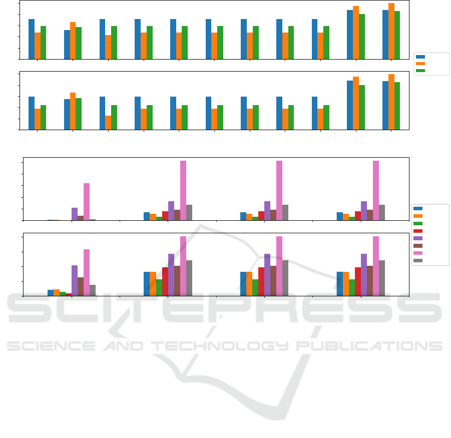
4 RESULTS AND DISCUSSIONS

Figure 4a. presents the metrics of classiﬁcation mod-

els computed on the respective test sets. The high-

est accuracy scores and F1 scores are obtained in

the cases of linear and quadrant discriminant analy-

ses across all the target classes. The tree-based al-

gorithms perform almost the same for the same class

with the logistic regression obtaining the least scores

in both metrics for all classes. The average best score

on the test sets across both metrics from the best per-

forming Quadratic Discriminant Analysis model for

classes DOC, Feed and Material are 87.54%, 100%

and 85.33% respectively.

Figure 4b. presents the regression model perfor-

mances. The AE samples having the same set of Ma-

terial, DOC and Feed present a comprehensivedataset

IN4PL 2021 - 2nd International Conference on Innovative Intelligent Industrial Production and Logistics

112

0.0

0.2

0.4

0.6

0.8

1.0

Accu racy

Log ist ic KNeigh bors SVC Gaussian Decision Tree Ran dom Forest MLP AdaBoost Naiv e Bay es LDA QDA

0.0

0.2

0.4

0.6

0.8

1.0

F1 Score

DOC

Feed

Mat erial

(a)

0.00

0.05

0.10

0.15

0.20

0.25

Mean Squared Error

Linear Lasso Elast ic Net LassoLars

0.0

0.1

0.2

0.3

0.4

Mean Absolut e Error

(1, 1, 9)

(1, 2, 12)

(1, 3, 11)

(1, 4, 10)

(2, 5, 16)

(2, 6, 15)

(2, 7, 13)

(2, 8, 14)

(b)

Figure 4: Model Performances (a) Classiﬁcation Models: AE vs DOC, Feed, Material (b) Regression Models: AE vs Tool

Wear.

to be able to predict tool wear under the same condi-

tions. As shown, the linear models show the lowest

mean absolute errors and mean squared errors across

all the datasets. This can be perhaps due to lower

number of recorded samples from the individual cases

across the two experiments. The average mean abso-

lute error on the test sets for linear models across the

cases is 0.1090 while the average mean squared error

is 0.03132.

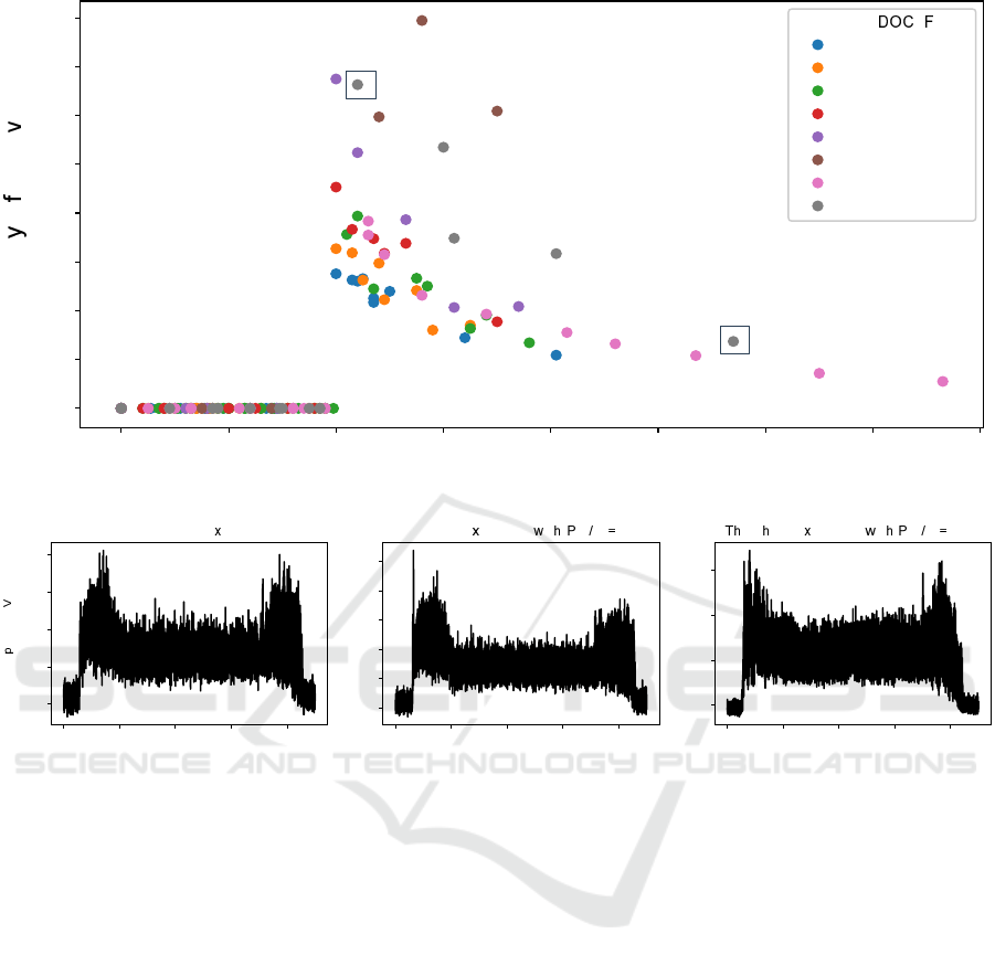
In Figure 5a., the distribution of events before and

after the set threshold t = 0.4 is exceeded can be seen.

The zero probabilities simply say that the correspond-

ing AE signal has not contributed to the threshold

crossing. The decreasing non-zero probabilities indi-

cate those events in which the tool wear has been af-

fected enough to cross the threshold. Higher probabil-

ities indicate greater tendency of deviating AE sam-

ples that lead to a higher amount of tool wear, while

the lower non-zero values can be interpreted as least

contributing towards further tool degradation, how-

ever this may change once more samples are obtained

and the tool wear amount increases for latter samples.

Once predicted tool wear values are obtained, these

can be included in the proposed distribution model

to visualize the possible degradations over the next

set of AE values if available. Temporal dependencies

are not used in this approach, which makes it a sim-

pler model to visualize next set of tool wear degra-

dation towards a wear limit beyond the set thresh-

old. In Figure 5a., two AE events are highlighted

(boxed) from the data-set corresponding to cast iron

material with a DOC value of 0.75 and Feed value

of 0.5. The corresponding AE signals are shown in

Figure 5b. where the signal exceeding the thresh-

old value 0.4 with a higher probability (center sig-

nal) is different from the immediate previous signal

where the threshold was not exceeded (left signal).

The AE signal where threshold was crossed but has

a least probability slightly differs from the remain-

ing two signals indicating lesser impact on tool wear

post the event where the threshold was actually ex-

ceeded with a higher probability. The combinations

of imputed targets and predicted target are valuable to

this model since the probabilities are calculated over

all the available samples. With lesser samples, this

model could lead to skewed values. For validation

Efﬁcacy of Statistical Formulations on Acoustic Emission Signals for Tool Wear Predictions

113

0.0 0.2 0.4 0.6 0.8 1.0 1.2 1.4 1.6

Tool Wear (cm )

0.00

0.05

0.10

0.15

0.20

0.25

0.30

0.35

0.40

Probabilit o AE E ent

(Mat erial, , eed)

(1, 1.5, 0.5)

(1, 0.75, 0.5)

(1, 0.75, 0.25)

(1, 1.5, 0.25)

(2, 1.5, 0.5)

(2, 1.5, 0.25)

(2, 0.75, 0.25)

(2, 0.75, 0.5)

(a)

0 2000 4000 6000 8000

0.10

0.15

0.20

0.25

0.30

Am lit ud e ( )

Threshold Not E ceeded

0 2000 4000 6000 8000

0.10

0.15

0.20

0.25

0.30

0.35

Threshold E ceeded it (A E) 0.33

0 2000 4000 6000 8000

0.1

0.2

0.3

0.4

res old E ceeded it (A E) 0.06

(b)

Figure 5: Comparisons of AE Events with Actual Signals (a) Progression of Tool Wear with every AE Event (b) AE Events

from Cases 8 and 14.

of such models, manual comparison with tools at that

stage where higher probabilities are predicted, is re-

quired, which has not been possible in this case due

to the use of public data-set.

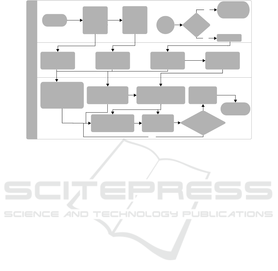
Figure 6. presents the outline of integration of

proposed statistical and prediction schemes in actual

industrial cases. Prediction softwares available com-

mercially can be used in addition to DAQ systems

where AE events are captured to simultaneous pro-

vide prognostic analysis when the machine is in pro-

cess. The use of modern embedded controllers such

as those provided by National Instruments (NI) can be

used to integrate this scheme in industrial scenarios.

5 CONCLUSIONS

Based on acoustic emissions, a mixedanalysis using a

statistical model and predictive models has been pro-

posed in this paper. The use of machine learning al-

gorithms presents a non-conventional approach to es-

tablish relations between emission samples from sen-

sors to observed tool wear. In cases where the tool

wear values were missing, an imputation scheme is

presented based on the behavior of tool wear. The

Bayesian model based on the calculated areas under

AE signals and tool wear values give a certain insight

into the pattern of approaching a threshold value for

manual inspection. Along with predicted tool wear

values, this scheme can be used to highlight the pro-

cess at a certain signal where higher probabilities in-

dicate the effect on tool wear has been signiﬁcant,

while lower probabilities are still open to interpreta-

tion. Based on these preliminary investigations, one

cannot claim to deﬁnitively stop the process where

tool is predicted to be highly impacted, but the meth-

ods can be validated and implemented on different

data-sets for variability. The current scheme may be

useful in prognostic cases where small samples of AE

data are extracted and used for analysis. However,

IN4PL 2021 - 2nd International Conference on Innovative Intelligent Industrial Production and Logistics

114

Machining

Process

Sensor

Placements

and

Conditions

Checked

Operator

Can the

process

begin

Check Process

and Monitoring

Parameters

Yes

Proceed

Machine Floor

Data Acquisition

System

Modeling System

Machining

Parameters

Set and

Conditions

Checked

Record

Machine Data

Record AE Data

Observe and

Calculate Tool

Wear

Data Imputation

using Domain

Rules

Classifications Models

to get relations

between AE data and

Tool Wear

Bayesian Models to infer

which AE reading crosses

threshold

Inspect Tool

and

Workbench

Regression Models to

predict Tool Wear

Predicted parameters,

tool wear readings

and Bayesian inflences

Observe the

readings with

Bayesian Model

Is any

reading crossing

threshold?

Exit

Monitoring

Yes

Figure 6: Integration of Prediction Models for Traceability.

with the proposed integration scheme using available

DAQ systems, analysis toolboxes and cloud based

data distribution, scalable implementations with big

data may also be possible. The predictive models can

also be compared with advanced neural network anal-

ysis along with variation in considered classes from

binary to multi-label problems. These directions are

planned in future works.

REFERENCES

Agogino, A. and Goebel, K. (2007). Milling data set.

Al-Jumaili, S. K., Pearson, M. R., Holford, K. M., Eaton,

M. J., and Pullin, R. (2016). Acoustic emission source

location in complex structures using full automatic

delta t mapping technique. Mechanical Systems and

Signal Processing, 72-73:513–524.

Bhuiyan, M., Choudhury, I. A., Dahari, M., Nukman, Y.,

and Dawal, S. Z. (2016). Application of acoustic emis-

sion sensor to investigate the frequency of tool wear

and plastic deformation in tool condition monitoring.

Measurement, 92:208–217.

Carpenter, S. H. and Zhu, Z. (1991). Correlation of the

acoustic emission and the fracture toughness of duc-

tile nodular cast iron. Journal of Materials Science,

26(8):2057–2062.

Chiementin, X., Mba, D., Charnley, B., Lignon, S., and

Dron, J. P. (2010). Effect of the denoising on acoustic

emission signals. Journal of Vibration and Acoustics,

132(3).

del Val, L., Izquierdo, A., Villacorta, J. J., and Su´arez, L.

(2020). Comparison of methodologies for the detec-

tion of multiple failures using acoustic images in fan

matrices. Shock and Vibration, 2020:1–10.

Du, F., Xu, C., Ren, H., and Yan, C. (2018). Structural

health monitoring of bolted joints using guided waves:

A review. In Wahab, M. A., Zhou, Y. L., and Maia,

N. M. M., editors, Structural Health Monitoring from

Sensing to Processing. InTech.

Grosse, C. and Ohtsu, M. (2008). Acoustic Emission Test-

ing. Springer Berlin Heidelberg, Berlin, Heidelberg.

Khan, M. T. I. (2018). Structural health monitoring by

acoustic emission technique. In Wahab, M. A., Zhou,

Y. L., and Maia, N. M. M., editors, Structural Health

Monitoring from Sensing to Processing. InTech.

Mokhtari, N., Pelham, J. G., Nowoisky, S., Bote-Garcia, J.-

L., and G¨uhmann, C. (2020). Friction and wear mon-

itoring methods for journal bearings of geared turbo-

fans based on acoustic emission signals and machine

learning. Lubricants, 8(3):29.

Niknam, S. A., Thomas, T., Hines, J. W., and Sawhney, R.

(2013). Analysis of acoustic emission data for bear-

ings subject to unbalance. International Journal of

Prognostics and Health Management, 4(3).

Pearson, M. R., Eaton, M., Featherston, C., Pullin, R.,

and Holford, K. (2017). Improved acoustic emission

source location during fatigue and impact events in

metallic and composite structures. Structural Health

Monitoring, 16(4):382–399.

Singh, K., Nagar, Y., Kapil, J., Satyawali, P., and Ganju, A.

(2012). Preliminary investigations of acoustics emis-

sion signal from snow and its wavelet transform. J.

Acoustic Emission, 30:100–108.

Suwansin, W. and Phasukkit, P. (2021). Deep learning-

based acoustic emission scheme for nondestructive lo-

calization of cracks in train rails under a load. Sensors

(Basel, Switzerland), 21(1).

Usgame, H., Pedraza, C., and Quiroga, J. (2013). Acoustic

emission-based early fault detection in tapered roller

bearings. Ingenier´ıa e Investigaci´on, 33(3):5–10.

Efﬁcacy of Statistical Formulations on Acoustic Emission Signals for Tool Wear Predictions

115