Optimizing Sales Forecasting in e-Commerce with ARIMA and LSTM

Models

Konstantinos N. Vavliakis

1,2

, Andreas Siailis

and Andreas L. Symeonidis

Department of Electrical and Computer Engineering, Aristotle University of Thessaloniki, Thessaloniki, GR54124, Greece

Pharm24.gr, Dafni Lakonias, GR23057, Greece

Keywords:

Sales Forecasting, e-Commerce, Neural Network, ARIMA, RNN.

Abstract:

Sales forecasting is the process of estimating future revenue by predicting the amount of product or services

a sales unit will sell in the near future. Although signiﬁcant advances have been made in developing sales

forecasting techniques over the past decades, the problem is so diverse and multi-dimensional that only in a

few cases high accuracy predictions can be achieved. In this work, we propose a new hybrid model that is

suitable for modeling linear and non-linear sales trends by combining an ARIMA (autoregressive integrated

moving average) model with an LSTM (Long short-term memory) neural network. The primary focus of

our work is predicting e-commerce sales, so we incorporated in our solution the value of the ﬁnal sale, as it

greatly affects sales in highly competitive and price-sensitive environments like e-commerce. We compare

the proposed solution against three competitive solutions using a dataset coming from a real-life e-commerce

store, and we show that our solution outperforms all three competing models.

1 INTRODUCTION

Sales forecasting is the process that enables a busi-

ness to estimate future sales. Inventory planning,

production scheduling, cash ﬂow planning, alignment

of sales quotas and revenue expectations as well as

other commercial decisions, all depend on the pre-

cision of forecasts. Sales forecasting adds value

across an organization as for proﬁtable retail busi-

nesses, accurate demand forecasting is crucial. Ac-

curate sales forecasting is of paramount importance to

e-commerce business (Qi et al., 2019), as e-commerce

sales are known to suffer from increased volatility,

unpredictability, and sudden spikes or lows, due to

abrupt changes in various source revenue channels,

like changes in organic trafﬁc, paid media, social

buzz, etc.

To produce sales forecasts, a multidisciplinary

group of information must be considered, such as

historical trends, pricing, customer data, promotions,

selling channels, and product changes. Moreover, one

must successfully anticipate market trends, monitor

competitors, and consider other business plans. Typ-

ically, sales have three long-term stages growth, sta-

bility, and decline (Day, 1981), while in short term

they are affected by price, promotions, season, and

online ranking. Especially in e-commerce environ-

ments, sales ﬂuctuations are sudden, blunt, and hard

to predict if not all underlying information is avail-

able. Thus, even though sales may show a linear trend

of increase or decrease in a speciﬁc period, certain

phases may show the characteristics of nonlinear ﬂuc-

tuation because of various potential uncertainties (Li

et al., 2018).

Various techniques can be used for forecasting,

like qualitative techniques, time series analysis and

projection, as well as causal models (Chambers et al.,

1971). The ﬁrst uses qualitative data, such as ex-

pert opinion and information about special events, and

may or may not consider the past. The second, on the

other hand, focuses entirely on patterns and pattern

changes, and thus relies entirely on historical data.

The third uses highly reﬁned and speciﬁc information

about relationships between system elements and is

powerful enough to take special events formally into

account. As with time series analysis and projection

techniques, the past is important to causal models. Se-

lecting the appropriate forecasting technique requires

evaluation of various parameters (Armstrong, 2009)

like accuracy, convenience, market popularity, appli-

cations, data required, and cost of forecasting.

Towards improving sales forecasting, various top-

down and bottom-up techniques have been proposed

(Soto-Ferrari et al., 2019) in the past. Top-down

Vavliakis, K., Siailis, A. and Symeonidis, A.

Optimizing Sales Forecasting in e-Commerce with ARIMA and LSTM Models.

DOI: 10.5220/0010659500003058

In Proceedings of the 17th International Conference on Web Information Systems and Technologies (WEBIST 2021), pages 299-306

ISBN: 978-989-758-536-4; ISSN: 2184-3252

299

sales forecasting starts by identifying your total ad-

dressable market for each business segment. It takes

a higher-level approach to view your business. On

the opposite spectrum is bottom-up sales forecasting,

which starts with the product instead of the market

and unit sales instead of market share. Bottom-up

forecasting, as well as sales forecasting by product,

is usually reserved for more mature businesses.

The ultimate goal of predictive analytics for sales

forecasting is to fully automate the forecasting pro-

cess and enable continuous forecasting with real-time

data. This is done by capturing and digitizing hu-

man expertise, essentially teaching a computer system

to “think” like a human sales planner, being able to

model both linear and non-linear variables. Towards

this end, various machine learning techniques have

been proposed, including statistical methods, time se-

ries analysis, neural networks, and random forests.

In this work, we propose an augmented hybrid

model that handles linear and non-linear relationships

for solving the problem of automatic product sales

forecasting. The proposed model handles univariate

timeseries predictions, to predict the future number of

sales, by integrating an ARIMA model with a state-

of-the-art neural network. In addition, the ﬁnal re-

tail price of the product is used as input in the neu-

ral network that improves the accuracy of the predic-

tions, as the e-commerce market usually is very price-

sensitive, so discounts and ﬁnal price greatly affect

sales.

The remainder of this paper is structured as fol-

lows. Section 2 discusses related work on sales fore-

casting, while Section 3 presents the proposed fore-

casting model. Section 4 depicts the results on the

evaluation process. Finally, Section 5 summarizes

work done, discusses future work, and concludes the

paper.

2 RELATED WORK

Although most sales forecasting techniques are typ-

ically univariate methods that produce forecasts con-

sidering only the historical sales data of a single prod-

uct, there is a lot more information that can be used

for improving forecasting models. Apart from the his-

torical trends, like sales from previous years, extra in-

formation can be utilized, like pricing, customer data,

promotion activity, sales channel differentiation, and

product changes, as well as market trends, competitor

analysis, and future business plans. Towards improv-

ing sales forecasting various top-down and bottom-up

techniques have been proposed in the past.

Statistical sales forecasting models like ARIMA

(Box and Pierce, 1970), can be identiﬁed as one of

the most traditional and commonly used forecasting

methodologies. ARIMA models are a class of statis-

tical models for analyzing and forecasting time series

data that have been widely used for sales forecasting.

Recently researchers (Ramos et al., 2015) compared

the forecasting performance of state-space models

and ARIMA models. The forecasting performance

was demonstrated through a case study of retail sales

of ﬁve different categories of women’s footwear. The

results of this work showed that when an automatic

algorithm is used, the overall out-of-sample forecast-

ing performance of state space and ARIMA models

evaluated via RMSE, MAE, and MAPE (Chai and

Draxler, 2014) is quite similar on both one-step and

multi-step forecasts. Ramos et al., (2015) also con-

cluded that state space and ARIMA produce cover-

age probabilities that are close to the nominal rates

for both one-step and multi-step forecasts. More-

over, ARIMA models were also combined (Li et al.,

2018) with autoregressive neural networks (ARIMA-

NARNN) for forecasting e-commerce sales. This

work showed that the ARIMA-NARNN model, which

combines the linear ﬁtting of ARIMA and the non-

linear mapping of NARNN, shows better prediction

performance than the ARIMA and NARNN methods.

Artiﬁcial neural networks (ANNs) have also been

widely used for forecasting models. A complete

framework was presented (Doganis et al., 2006) that

can be used for developing nonlinear time series sales

forecasting models. This method combined two arti-

ﬁcial intelligence technologies, namely the radial ba-

sis function (RBF) neural network architecture, and

a specially designed genetic algorithm (GA). Situ-

ations where large quantities of related time series

are available have also been investigated (Bandara

et al., 2019) and results showed that conditioning the

forecast of an individual time series on past behav-

ior of similar, related time series can be beneﬁcial.

Bandara et al. (2019) attempted to incorporate the

product assortment hierarchy in an e-commerce plat-

form that contained large numbers of related prod-

ucts, to a uniﬁed model. They trained a Long Short-

Term Memory network (Hochreiter and Schmidhu-

ber, 1997) that exploited the non-linear demand re-

lationships available in an e-commerce product as-

sortment hierarchy. They also proposed a systematic

pre-processing framework to overcome the challenges

in the e-commerce business. Finally, they intro-

duced several product grouping strategies to supple-

ment the LSTM learning schemes, in situations where

sales patterns in a product portfolio were disparate.

Novel neural networks called extreme learning ma-

WEBIST 2021 - 17th International Conference on Web Information Systems and Technologies

300

chine (ELM) have also been investigated (Sun et al.,

2008) in order to ﬁnd the relationship between sales

amount and some signiﬁcant factors which affect de-

mand (such as design factors). Sun et al. (2008) used

real data from a fashion retailer to demonstrate that

the proposed methods outperform several sales fore-

casting methods which are based on backpropagation

neural networks.

Although ARIMA was one of the popular lin-

ear models in time series forecasting during the past

three decades. Recent research activities in forecast-

ing with artiﬁcial neural networks (ANNs) suggested

that ANNs can be a promising alternative to the tra-

ditional linear methods. Towards this end, ARIMA

models and ANNs are often compared with mixed

conclusions in terms of the superiority in forecasting

performance (Zhang, 2003). Since there are conﬂict-

ing studies about the superiority or not of neural net-

works, when compared with ARIMA models, hybrid

methods have also been proposed.

Zhang, (2003) proposed a hybrid methodology

that combines both ARIMA and ANN models that

take advantage of the unique strength of ARIMA and

ANN models in linear and nonlinear modeling. Ex-

perimental results with real data sets indicate that the

combined model can be an effective way to improve

forecasting accuracy achieved by either of the mod-

els used separately. On the other hand, a hybrid

forecasting method that also been proposed (Khan-

delwal et al., 2015) that applies ARIMA and ANN

separately to model linear and nonlinear components,

respectively after a prior decomposition of the se-

ries into low and high-frequency signals through dis-

crete wavelet transformation. These empirical results

with four real-world time series demonstrated that

the proposed method has yielded better forecasts than

ARIMA, ANN, and Zhang’s hybrid (Zhang, 2003)

model.

Other techniques, like multivariate methods, have

also been used. Fan et al., (2017) used online re-

views and a sentiment analysis method, the Naive

Bayes algorithm, to extract the sentiment index from

the content of each online review and integrate it into

the imitation coefﬁcient of the Bass Norton model

to improve the forecasting accuracy. Their compu-

tational results indicated that the combination of the

Bass/Norton model and sentiment analysis has higher

forecasting accuracy than the standard Bass/Norton

model and some other sales forecasting models. On

the other hand, Lu et al., (2012) used multivari-

ate adaptive regression splines (MARS), a nonlinear

and nonparametric regression methodology, to con-

struct sales forecasting models for computer whole-

salers. Their experimental results show that the

MARS model outperforms backpropagation neural

networks, a support vector machine, a cerebellar

model articulation controller neural network, an ex-

treme learning machine, an ARIMA model, a mul-

tivariate linear regression model, and four two-stage

forecasting schemes across various performance cri-

teria. Guo et al., (2013) effectively applied multivari-

ate intelligent decision-making (MID) model and de-

veloped an effective forecasting model for the prob-

lem of sales forecasting problem in the retail industry

by integrating a data preparation and preprocessing

module, a harmony search-wrapper-based variable se-

lection (HWVS) module, and a multivariate intelli-

gent forecaster (MIF) module. Their experimental re-

sults showed that it is statistically signiﬁcant that the

proposed MID model can generate much better fore-

casts than machine learning models and generalized

linear models do.

Other machine learning models have also been

employed frequently as they were able to achieve bet-

ter results using non-linear data. The recent research

shows that deep learning models (e.g., recurrent neu-

ral networks) can provide higher accuracy in predic-

tions compared to machine learning models due to

their ability to persist information and identify tem-

poral relationships. A study of deep learning-based

models for forecasting future directions of car sales

has also been proposed (Preeti Saxena, 2020). The re-

sults of this model based on ARIMA and Long Short-

Term Memory-Recurrent Neural Network (LSTM-

RNN) based models are analyzed and used for fore-

casting future directions. Their results showed that

LSTM-RNN is better than the ARIMA for the multi-

variate datasets.

Multi-disciplinary efforts have also been pre-

sented. Gurnani et al., (2017) evaluate and compares

various machine learning models, namely, ARIMA,

Auto-Regressive Neural Network (ARNN), XGBoost

(Chen and Guestrin, 2016), SVM (Hearst et al.,

1998), Hybrid Models like Hybrid ARIMA-ARNN,

Hybrid ARIMA-XGBoost, Hybrid ARIMA-SVM,

and STL Decomposition (Theodosiou, 2011), using

ARIMA, Snaive and XGBoost, to forecast sales of

a drug store. The accuracy of these models was

measured by metrics such as MAE and RMSE. Ini-

tially, a linear model such as ARIMA has been ap-

plied to forecast sales. But ARIMA was not able to

capture nonlinear patterns precisely, hence nonlinear

models such as Neural Network, XGBoost, and SVM

were used. Nonlinear models performed better than

ARIMA and gave lower RMSE. Then, to further op-

timize the performance, composite models were de-

signed using the hybrid technique and decomposition

technique. Hybrid ARIMA-ARNN, Hybrid ARIMA-

Optimizing Sales Forecasting in e-Commerce with ARIMA and LSTM Models

301

XGBoost, Hybrid ARIMA-SVM were used and all of

them performed better than their respective individual

models. The composite model was designed using

STL Decomposition where the decomposed compo-

nents namely seasonal trend, and remainder compo-

nents were forecasted by Snaive, ARIMA, and XG-

Boost. STL gave better results than individual and

hybrid models.

It is obvious that a lot of research efforts try to ana-

lyze and improve sales forecasting systems dynamics;

however, most of the existing solutions focus on spe-

ciﬁc case studies or ofﬂine retailers. Although dur-

ing the last years research focus has been shifted to

e-commerce, there is still a lot of progress to be made

for accurately forecasting sales. Moreover, most of

the proposed solutions focus on products and properly

forecasting their sales over time based on linear sales

data, while when non-linear or hybrid approaches

have been proposed, they rely on one-dimensional

data. In this work, we extend the current state of the

art by proposing a) a hybrid sales forecasting model

for dynamic pricing that optimally integrated ARIMA

and LSTM models, and b) integrates sales data with

pricing information for improved forecasting results.

3 PROPOSED SOLUTION

Our proposed solution is a hybrid model that

combines an ARIMA model for forecasting one-

dimensional time series data and an LSTM neural

network that models the non-linear residuals of the

ARIMA model together with the ﬁnal retail price (re-

tail price after discounts). Selling price is a major

factor that affects sales, especially in highly compet-

itive environments, like e-commerce, thus our model

captures special discounts, promotions, and sales pe-

riods by the integration of the retail price, after dis-

counts, in our model. Moreover, trends and season-

ality are captured by the ARIMA time series analysis

of the proposed system. Our proposed model extends

the work of Zhang, (2003) by a) using state-of-the-art

neural model (LSTM) and b) extending the univari-

ate approach of Zhang into multivariate by using the

average retail selling price.

A time series y

is composed of a linear L

and a

non-linear component N

, according to Equation 1.

= L

+ N

(1)

The ARIMA methodology models the L

compo-

nent and the LSTM neural network models what can-

not be modeled by the linear ARIMA model, that is

the N

component. We call e

the non-linear informa-

tion until timestep t, so: e

= y

−

, where

is the

prediction from the ARIMA model until timestep t.

The input of the LSTM model is the non-linear resid-

uals that are not modeled from the ARIMA model.

In addition, we add another input which is the av-

erage ﬁnal retail price of each product at timestep t,

as in Equation 2 where f is the non-linear function

that will be modeled by the LSTM, having as inputs

the ARIMA residuals and retail price for the last n

timesteps.

ˆe

= f (e

t−1

, e

t−2

, . . . , e

t−n

, p

t−1

, p

t−2

, . . . , p

t−n

) (2)

Figure 1 depicts the system architecture of the pro-

posed solution. The pre-processing phase includes

data cleaning, sorting, and indexing based on the date

sold. Since ARIMA models are suitable only for one-

dimensional time series analysis, we use as an input

only the quantity sold for n timesteps. The ARIMA

modeling function is depicted in Equation 3.

ˆy

= µ + φ

t−1

+ ... + φ

t−p

t−1

+ ... + θ

t−q

(3)

Where y

t−1

...y

t−p

are the selling quantities for

p previous timesteps (autoregressive parameters) and

t−1

...e

t−q

are the moving average parameters that re-

fer to external factors for the previous q timesteps.

Factors φ

...φ

and θ

...θ

are the trained autoregres-

sive parameters and moving average parameters, re-

spectively. This process is repeated for d times.

The values of (p, d, q) that lead to the optimal re-

sults are different for each product, thus optimiza-

tion of (p, d, q) must take place to discover the op-

timal values that lead to the best MSE (mean square

error). After that, data prediction takes place to

model the residuals, which is the difference be-

tween the actual and predicted values (Residuals =

Actual–Prediction). Two are the factors that indicate

a good prediction: a) the residuals are unrelated; thus,

we cannot ﬁnd a relation between residuals that we

could use for improving prediction results, and b) the

residuals mean value is close to zero, thus the stan-

dard deviation between predicted and real values is

minimum.

After the ARIMA model is completed, the residu-

als together with the ﬁnal price are normalized using

the min-max scaling technique (Equation 4) and they

are fed to the LSTM network.

(x − x

min

)

max

− x

min

)

(4)

Next, we calculate the optimal number of time

lags, as well as the number of hidden neurons,

together with numerous other parameters such as

nE pochs, nSamples, batchSize, learningRate, loss

function, and activation function using a grid-search

WEBIST 2021 - 17th International Conference on Web Information Systems and Technologies

302

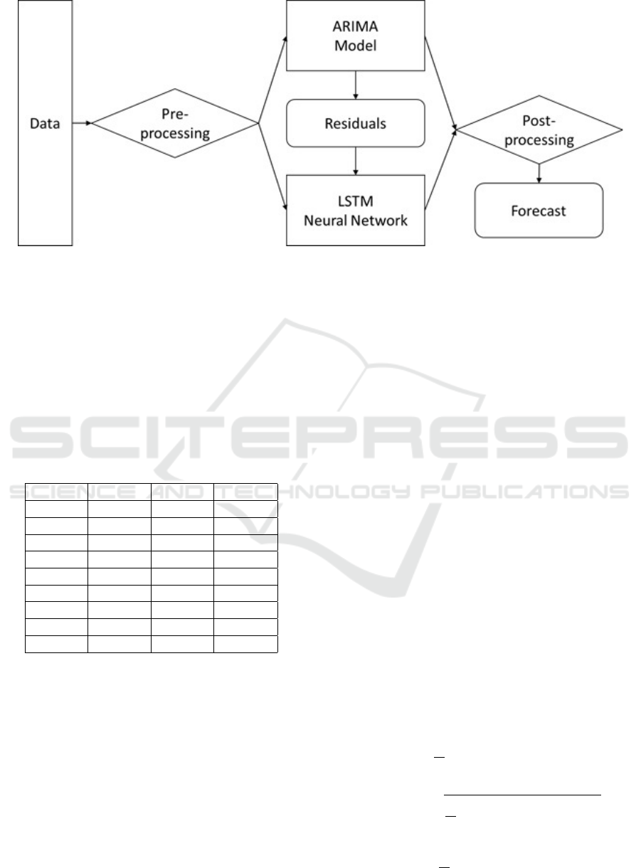
Figure 1: Architectural diagram of the proposed solution.

technique with various parameters and then the

LSTM network, is ready for our predictions. Since

the LSTM network calculates the diversion between

the real sales quantity and the value predicted by the

ARIMA model the ﬁnal sales prediction is depicted

in Equation 5.

FinalPrediction = Prediction

ARIMA

−Prediction

LST M

(5)

Table 1: Example Results for Grid Search of Optimum Val-

ues for (p, q, d).

(p, q, d) MSE (p, q, d) MSE

(1,0,0) 86.152 (4,0,0) 107.509

(1,0,1) 86.950 (4,0,1) 96.286

(1,1,0) 51.191 (4,1,0) 91.419

(2,0,0) 95.040 (4,1,1) 89.248

(2,1,0) 53.616 (4,1,2) 110.837

(3,0,0) 106.914 (5,0,0) 104.366

(3,1,0) 71.840 (5,1,0) 82.534

(3,1,1) 90.332 (5,1,1) 83.516

(3,1,2) 92.695 (5,1,2) 84.089

4 EVALUATION

4.1 Evaluation Data

For evaluation, we used an anonymous dataset

from the Greek online pharmacy www.pharm24.gr.

Pharm24.gr which is a well-known online pharmacy

in Greece with a few hundred thousand visitors per

month. Although considerably smaller than the global

e-commerce giants, Pharm24.gr just like many more

small-medium e-commerce retailers, has enough traf-

ﬁc and revenue to justify some research & develop-

ment for optimizing sales predictions, provided the

applied methods use limited resources. Our dataset

contained selling data for 23,432 products, spanning

over six years and 1,418,480 order lines. For each

product, we used the quantities sold per month and

the average retail price per month.

Pre-processing has to take place in order to con-

vert data to the appropriate format for the ARIMA

model. During pre-processing the following steps are

taken: a) sales data are ordered by datetime, b) data

are reduced to one-dimensional information, so extra

information like average price and other product at-

tributes are removed, and c) dates with zero sales are

ﬁlled in order to have equal sized timeseries.

4.2 Evaluation Metrics

For evaluation we used three metrics: a) Mean Square

Error (MSE), b) Root Mean Square Error (RMSE),

and c) Mean Absolute Error (MAE) according to

Equations 6, 7, and 8 respectively, where pred

f inal

the ﬁnal prediction values as calculated by the com-

bination of the results of the ARIMA model and the

LSTM network for timeframe i, actual

is the actual

quantities sold in timeframe i and N is the number of

forecasting timeframes.

MSE =

∑

i=1

(actual

− pred

f inal

)

(6)

RMSE =

∑

i=1

(actual

− pred

f inal

)

(7)

MAE =

∑

i=1

|actual

− pred

f inal

| (8)

Optimizing Sales Forecasting in e-Commerce with ARIMA and LSTM Models

303

Table 2: Evaluation of our solution against the results of the ARIMA model, the LSTM network, and the Zhang hybrid model

for one product.

Actual

ARIMA

Prediction

LSTM

Prediction

Zhang

Prediction

of the

Proposed Model

Month Quantity

Sold

1 19 10.042152 9.404712 12.200262 13.566653

2 6 11.821504 8.800409 11.237559 14.334739

3 25 11.247403 10.811686 12.549486 15.364458

4 19 15.037372 10.380136 14.679003 21.467420

5 25 18.728056 13.610783 18.885234 21.285071

6 18 15.972515 18.334824 15.079795 18.489854

7 19 15.211719 15.827807 14.937994 19.230617

8 13 14.377784 16.447681 14.430467 16.174313

9 14 12.831789 13.638979 13.167471 14.847084

10 12 11.790429 12.937215 11.285167 14.855980

11 22 12.453913 11.919153 12.391926 15.389440

12 12 16.381802 14.070756 15.835681 18.792803

In order to optimize the (p, d, q) values, as dis-

cussed in Section 3, we applied a grid search (Lerman,

1980) optimization algorithm for p = [0, 1, 2, 3, 4, 5],

d = [0, 1], and q = [0, 1, 2], where p is the number

of AR terms, d is the number of iterations for cal-

culating the residual values and q in the number of

MA. Table 1 depicts some examples of our tests.

The initial search values were careful selected by a

domain expert and then we applied grid search that

gave the optimal results for (p, d, q) = (2, 1, 2), fur-

thermore we set the number of epochs equal to 1000

(nE pochs = 1000).

Next, we optimized the LSTM model. We con-

sidered two different methods, batch learning and on-

line learning that follow a different training method.

Gradient descent training of neural networks can be

done in either a batch or on-line manner. Wilson and

Martinez, (2003) explained why batch training is al-

most always slower than on-line training, often or-

ders of magnitude slower, especially on large train-

ing sets. The main reason is due to the ability of

on-line training to follow curves in the error surface

throughout each epoch, which allows it to safely use

a larger learning rate and converge with less iterations

through the training data. Thus, we decided to use

online learning (batch size = 1).

For optimizing the LSTM weights, we used the

ADAM method, an algorithm for ﬁrst-order gradient-

based optimization of stochastic objective functions,

based on adaptive estimates of lower-order moments

(Kingma and Ba, 2014), with the Keras (Ketkar,

2017) default values [learning rate = 0.001, beta 1 =

0.9, beta 2 = 0.999, epsilon = 1e − 07] and the rec-

tiﬁed linear activation function (ReLU) (Agarap,

2019).

4.3 Evaluation Results

Next, we compared the results of our solution against

the results of a) the ARIMA model, b) the LSTM

network, and c) the Zhang’s hybrid model. Table 2

depicts the results of the evaluation process for one

product.

We performed the above experiment for 50 ran-

dom products and then, we calculated MSE, RMSE,

and MAE. The aggregated results are depicted in

Table 3, according to which the proposed model

achieved improved results when compared with any

of the ARIMA, LSTM or Zhang’s approaches, even

when we did not consider the retail price sold. Our

results further improved, and outperformed in all met-

rics all three competing models, by achieving 5.82%,

13.12%, and 1.84% improved RMSE, 5.29%, 9.88%,

and 0.39% improved MAE, and 11,44%, 23,67%,

and 5,88% improved MSE when compared with the

ARIMA model, LSTM, and Zhang’s model, respec-

tively.

In our ﬁrst set of experiments, we noticed that

results were better on products with increased sales,

which is attributed to the fact that the LSTM network

requires a lot of data for proper training. Thus, we

performed two more experiments, where, instead of

randomly picking 50 products, we tested, in the ﬁrst

case with the 10 best seller products and the second

case with the 10 worst seller products (with a min-

imum of 50 items sold). In the case of best seller

products, the results of the proposed system further

improved by 2.22% and 1.71% in terms of RMSE and

MAE, respectively

Finally, in order to test the adaptability of our so-

lution, we selected 10 products with high seasonal-

WEBIST 2021 - 17th International Conference on Web Information Systems and Technologies

304

Table 3: Evaluation results for 50 products.

MSE RMSE MAE

LSTM 540.76758 13.2629 9.68830

ARIMA 466.05542 12.2340 9.21864

Baseline (Zhang) 438.51756 11.7378 8.76454

Proposed Methodology 415.44138 11.6794 8.88266

Proposed Methodology with Retail Price 412.74034 11.5222 8.73078

Table 4: Evaluation results for best sellers and worst sellers when compared with the baseline.

Improvement for

Best sellers

Improvement for

Worst Sellers

Improvement for

Seasonal Products

MSE 5.81% 0.27% 4.11%

RMSE 2.22% 0.15% 1.76%

MAE 1.71% 0.3% 0.92%

ity (sunscreens). The results of all these three exper-

iments are depicted in Table 4. In all three cases, the

proposed solution outperformed the baseline, as we

achieved a 1.76% improvement in RMSE, 0.92% im-

provement in MAE and 4.11% improvement in MSE

when compared with the Zhang’s model.

5 CONCLUSIONS & FUTURE

WORK

In this paper, we introduced a novel sales forecast-

ing model that is based on a hybrid model. We com-

bined an ARIMA model that is suitable for linear

data, with an LSTM Network that analyses the non-

linear residuals of the ARIMA model. We also added

to our model an extra feature, the average retail sales

price, which naturally has a signiﬁcant effect on sales

volume, especially in highly price-sensitive environ-

ments, like the e-commerce ﬁeld.

We compared the proposed solution with three

other methods: a) the ARIMA model, b) the LSTM

model, and c) the Zhang model. Our solution out-

performed all three models by achieving improved

RMSE, MAE, and MSE when compared with the

ARIMA model, LSTM and Zhang’s model, respec-

tively. We stated that our model works better when

there is a plethora of data (due to the LSTM network),

so we performed another experiment with the best

seller products and the results of the proposed sys-

tem further improved by 2.22% in terms of RMSE. Fi-

nally, we tested our system with ten random seasonal

products, where we achieved 1.76% improvement in

RMSE when compared with the Zhang’s model.

Our future work includes further testing the pro-

posed algorithm in real-world scenarios and improv-

ing our simulation framework in terms of available

conﬁgurations and extra features (e.g. out of stock

periods, web trafﬁc sources, customer proﬁle and

one time promotional products). Finally, our plans

include comparing the proposed system with more

sales forecasting models, as well as other available

datasets.

ACKNOWLEDGEMENTS

This research is co-ﬁnanced by Greece and the Eu-

ropean Union (European Social Fund - ESF) through

the Operational Programme ”Human Resources. De-

velopment, Education and Lifelong Learning” in the

context of the project ”Reinforcement of Postdoctoral

Researchers - 2nd Cycle” (MIS-5033021), imple-

mented by the State Scholarships Foundation (IKY).

The authors would also like to thank Kostas Niko-

laros of Pharm24.gr for his valuable feedback regard-

ing sales trends.

REFERENCES

Agarap, A. F. (2019). Deep learning using rectiﬁed linear

units (relu).

Armstrong, J. (2009). Selecting forecasting methods. SSRN

Electronic Journal.

Bandara, K., Shi, P., Bergmeir, C., Hewamalage, H., Tran,

Q., and Seaman, B. (2019). Sales demand forecast in

e-commerce using a long short-term memory neural

network methodology. In Gedeon, T., Wong, K. W.,

and Lee, M., editors, Neural Information Processing,

pages 462–474, Cham. Springer International Pub-

lishing.

Box, G. E. P. and Pierce, D. A. (1970). Distribution of resid-

ual autocorrelations in autoregressive-integrated mov-

ing average time series models. Journal of the Ameri-

can Statistical Association, 65(332):1509–1526.

Chai, T. and Draxler, R. (2014). Root mean square er-

ror (rmse) or mean absolute error (mae)?– arguments

Optimizing Sales Forecasting in e-Commerce with ARIMA and LSTM Models

305

against avoiding rmse in the literature. Geoscientiﬁc

Model Development, 7:1247–1250.

Chambers, J. C., Mullick, S. K., and Smith, D. D. (1971).

How to choose the right forecasting technique. Har-

vard Business Review.

Chen, T. and Guestrin, C. (2016). Xgboost: A scalable

tree boosting system. In Proceedings of the 22nd

ACM SIGKDD International Conference on Knowl-

edge Discovery and Data Mining, KDD ’16, page

785–794, New York, NY, USA. Association for Com-

puting Machinery.

Day, G. S. (1981). The product life cycle: Analysis and

applications issues. Journal of Marketing, 45(4):60–

67.

Doganis, P., Alexandridis, A., Patrinos, P., and Sarimveis,

H. (2006). Time series sales forecasting for short

shelf-life food products based on artiﬁcial neural net-

works and evolutionary computing. Journal of Food

Engineering, 75(2):196–204.

Hearst, M., Dumais, S., Osuna, E., Platt, J., and Scholkopf,

B. (1998). Support vector machines. IEEE Intelligent

Systems and their Applications, 13(4):18–28.

Hochreiter, S. and Schmidhuber, J. (1997). Long short-term

memory. Neural Computation, 9(8):1735–1780.

Ketkar, N. (2017). Introduction to Keras, pages 97–111.

Apress, Berkeley, CA.

Khandelwal, I., Adhikari, R., and Verma, G. (2015). Time

series forecasting using hybrid arima and ann mod-

els based on dwt decomposition. Procedia Computer

Science, 48:173–179. International Conference on

Computer, Communication and Convergence (ICCC

2015).

Kingma, D. and Ba, J. (2014). Adam: A method for

stochastic optimization. International Conference on

Learning Representations.

Lerman, P. M. (1980). Fitting segmented regression models

by grid search. Journal of the Royal Statistical Soci-

ety: Series C (Applied Statistics), 29(1):77–84.

Li, M., Ji, S., and Liu, G. (2018). Forecasting of Chinese

E-Commerce Sales: An Empirical Comparison of

ARIMA, Nonlinear Autoregressive Neural Network,

and a Combined ARIMA-NARNN Model. Mathemat-

ical Problems in Engineering, 2018:1–12.

Preeti Saxena, Pritika Bahad, R. K. (2020). Long short-term

memory-rnn based model for multivariate car sales

forecasting. International Journal of Advanced Sci-

ence and Technology, 29(04):4645 –.

Qi, Y., Li, C., Deng, H., Cai, M., Qi, Y., and Deng, Y.

(2019). A deep neural framework for sales forecast-

ing in e-commerce. In Proceedings of the 28th ACM

International Conference on Information and Knowl-

edge Management, CIKM ’19, page 299–308, New

York, NY, USA. Association for Computing Machin-

ery.

Ramos, P., Santos, N., and Rebelo, R. (2015). Performance

of state space and arima models for consumer retail

sales forecasting. Robotics and Computer-Integrated

Manufacturing, 34:151–163.

Soto-Ferrari, M., Chams-Anturi, O., Escorcia-Caballero,

J. P., Hussain, N., and Khan, M. (2019). Evaluation

of bottom-up and top-down strategies for aggregated

forecasts: State space models and arima applications.

In Paternina-Arboleda, C. and Voß, S., editors, Com-

putational Logistics, pages 413–427, Cham. Springer

International Publishing.

Sun, Z.-L., Choi, T.-M., Au, K.-F., and Yu, Y. (2008). Sales

forecasting using extreme learning machine with ap-

plications in fashion retailing. Decision Support Sys-

tems, 46(1):411–419.

Theodosiou, M. (2011). Forecasting monthly and quar-

terly time series using stl decomposition. Interna-

tional Journal of Forecasting, 27(4):1178–1195.

Zhang, G. (2003). Time series forecasting using a hybrid

arima and neural network model. Neurocomputing,

50:159–175.

WEBIST 2021 - 17th International Conference on Web Information Systems and Technologies

306

REFERENCES

Agarap, A. F. (2019). Deep learning using rectified linear