Characterizing N-Dimension Data Clusters:

A Density-based Metric for Compactness and Homogeneity Evaluation

Dylan Molini

and Kurosh Madani

LISSI Laboratory EA 3956, Universit

e Paris-Est Cr

eteil, Senart-FB Institute of Technology,

Campus de S

enart, 36-37 Rue Georges Charpak, F-77567 Lieusaint, France

Keywords:

Space Partitioning, Sub-spaces, Cluster’s Density, Industry 4.0, Cognitive Systems.

Abstract:

The new challenges Science is facing nowadays are legion; they mostly focus on high level technology, and

more speciﬁcally Robotics, Internet of Things, Smart Automation (cities, houses, plants, buildings, etc.), and

more recently Cyber-Physical Systems and Industry 4.0. For a long time, cognitive systems have been seen

as a mere dream only worth of Science Fiction. Even though there is much to be done, the researches and

progress made in Artiﬁcial Intelligence have let cognition-based systems make a great leap forward, which

is now an actual great area of interest for many scientists and industrialists. Nonetheless, there are two main

obstacles to system’s smartness: computational limitations and the inﬁnite number of states to deﬁne; Machine

Learning-based algorithms are perfectly suitable to Cognition and Automation, for they allow an automatic –

and accurate – identiﬁcation of the systems, usable as knowledge for later regulation. In this paper, we discuss

the beneﬁts of Machine Learning, and we present some new avenues of reﬂection for automatic behavior

correctness identiﬁcation through space partitioning, and density conceptualization and computation.

1 INTRODUCTION

While the XIX

century is that of industrial pro-

cesses and the beginning of production line, and the

century is characterized by mass production

and assembly line, the actual XXI

century is that

of Robotics, Automation and Hyper-Connectivity. A

great many of projects related to these topics are

current active areas of research: self-driving vehi-

cles

(Shan and Englot, 2018), domotics, exoskele-

tons, smart robots able to interact with human beings

(Russo, 2020), self-adaptable systems, telecommuni-

cations (IoT, 5G), etc.

Robotics and Automation are getting more and

more accurate and reliable; there are two ways to

achieve great performances: 1- By deﬁning explic-

itly how a system should behave in a certain context

(Expert System paradigm); 2- By letting the system

learn by itself and self-adapt through examples and

observations (Machine Learning paradigm).

The former has been considered so far as the most

reliable, since every possible state the system can en-

ter in is explicitly deﬁned by some experts or users;

https://orcid.org/0000-0002-6499-3959

Automated Vehicle AV and Advanced Driver Assis-

tance Systems ADAS as well.

nonetheless, it suffers from a severe limitation: deﬁn-

ing any possible behavior is an unfeasible task, and

thus severely hinders the self-adaptation capability.

A piece of solution comes along a possible usage

of the examples encountered by the system in order to

let it study from them and learn how to react in the al-

ready known contexts. Once more, encountering any

possible situation is merely unfeasible; it is though

greatly easier to cover many more cases through ob-

servations and experience than to list them manually.

Letting the system learn ever more through time al-

lows to hypothetically cover any possible scenario.

It is the Machine Learning ML paradigm; it can

be used to identify, characterize and eventually model

a system, what can serve several purposes, among

which its monitoring and its semi-manual regulation.

In general, the ﬁrst step of any ML-based identiﬁ-

cation technique is an exploration of the data to point

out what can be. This procedure is often blind – un-

supervised – and is processed to automatically extract

information from the data. The most common Data

Mining task is space-partitioning, also called cluster-

ing, which consists in gathering the data into compact

groups within those they share similarities. This step

can be used to identify the system’s local behaviors,

optimize the processes by gathering similar tasks, etc.

Molinié, D. and Madani, K.

Characterizing N-Dimension Data Clusters: A Density-based Metric for Compactness and Homogeneity Evaluation.

DOI: 10.5220/0010657500003062

In Proceedings of the 2nd International Conference on Innovative Intelligent Industrial Production and Logistics (IN4PL 2021), pages 13-24

ISBN: 978-989-758-535-7

A great area of interest for clustering could be the

modeling of a system. Indeed, each cluster should

contain similar data and thus can be assumed to rep-

resent a local behavior: a local model can therefore

be built upon it. This is the Multi-Models paradigm.

This decomposition of the feature space, and thus of

the system as a whole, is very suitable to an Automa-

tion and Industry 4.0 application; indeed, the corner-

stone of any network – such as an Industry 4.0 Cyber-

Physical System – is to treat every unit as a part of a

wider process. Clustering could help to identify the

elementary units of an industrial system, either phys-

ically (subprocesses) or theoretically (behaviors).

There exists plenty of clustering methods, but they

do not all perform alike. Their accuracy greatly de-

pends on the studied data; as such, two clustering al-

gorithms can be similar while achieving very differ-

ent results. The remaining question would be to know

how to automatically distinguish a good decomposi-

tion from a poor one. This knowledge can be very im-

portant and relevant for the further steps of the mod-

eling process; indeed, how to expect a good model

when the ﬁrst step, i.e. clustering, has achieved poor

results, and has gathered (very) dissimilar data?

In this paper, we will present a new way to quan-

tify the compactness of a cluster of data, which is very

useful as an indicator of data homogeneity. In the next

section, we will present both some Machine Learning

models and some Machine Learning-based clustering

methods; in section 3, we will detail both that used

and our homogeneity quantiﬁer. Section 4 will dis-

play some examples of results and how one can in-

terpret them for further understanding of the systems.

Finally, section 5 is the conclusion of this paper.

2 STATE OF THE ART

Whether it is artiﬁcial or biological (brain), a Neural

Network NN is somehow a graph where the nodes are

a sort of activator and the branches linking the nodes

to one another are a channel, whose span lets a signal

go through with a high or low amplitude, like a nozzle

would do. By analogy with the brain, the nodes are

called the neurons and the channels are the synapses.

Training an Artiﬁcial Neural Network means to

adapt ”the span” of its channels; a weighting coefﬁ-

cient (called weight) is responsible for this adaptation,

which is modiﬁed in such a way it ﬁts the known data.

More generally, the Machine Learning paradigm

exploits data and experience to train a system, and

to teach it how to behave within certain situations.

It relies on several approaches: Multi-Layer Percep-

tron MLP (Rumelhart et al., 1986a), Radial Basis

Function RBF (Broomhead and Lowe, 1988), Multi-

Expert System MES (Thiaw, 2008), Multi-Agent Sys-

tem MAS (Rumelhart et al., 1986b), Support Vector

Machine SVM (Boser et al., 1996), etc. The most

common model in use is the MLP, which is somehow

a representation of the biological brain; they are often

long to train however. Thus, some other models can

be preferred, depending on the context of application.

Though less widespread, another paradigm in use

is the Multi-Expert System MES: it is anew a Neural

Network, with the main difference that the neurons

are local experts. The output of the whole model is a

combination of the outputs of the local models. It is

an extension of the very widespread Expert System

paradigm (Buchanan and Feigenbaum, 1978). The

local experts can take many shapes, from expert sys-

tems to Machine Learning-based models (MLP, RBF,

SVM, etc.). Though still depending on the data and

on the context, MESs are capable of achieving great

accuracy, for the sub-models are trained to correctly

model and represent each of the system’s sub-parts.

As a consequence, to use the MES paradigm,

the feature space must be split upstream. As such,

we need a clustering method to make the framework

ready for this step. There exists several clustering

algorithms, mostly based on Machine Learning; this

avoids to have to rely on human experts charged to

manually describe the system, what can be hard and

time-greedy. Machine Learning lets a (smart) algo-

rithm do the job instead; the inquiry is mainly to know

whether or not one can trust the so-obtained clusters.

Once more, clustering can be driven by some

knowledge – supervised learning – or be totally blind

– unsupervised learning. However, supervised learn-

ing requires some often manual expertise of the data

(or given by an unsupervised algorithm upstream) and

is therefore not suitable to a blind data mining pro-

cedure. Among the existing clustering algorithms,

it is worth mentioning: K-Means (Jain, 2010), Self-

Organizing Maps (Kohonen, 1982), Neural Gas (Mar-

tinetz and Schulten, 1991), Fuzzy Clustering (Dunn,

1973) and Support Vector Machine (Boser et al.,

1996). The ﬁrst three are unsupervised, and are per-

fectly suitable to a data mining application.

The K-Means iteratively aggregate the data points

around some ”seeds” (random points drawn from the

database), and update them again and again until

satisfying some criterion. They are easy to imple-

ment, but are unable to cluster nonlinearly separable

datasets. The Kernel K-Means use a kernel (a pro-

jection of the data from an Euclidean space into a

non-Euclidean one, called kernel space) to compen-

sate that, but they are very resource-consuming and

are prone to achieve only local optima.

IN4PL 2021 - 2nd International Conference on Innovative Intelligent Industrial Production and Logistics

The Self-Organizing Maps are an ingenious exten-

sion of the K-Means, by linking the seeds with each

other, forming somehow a grid; it is now the whole

grid which is updated to ﬁt any data. They converge

quicker, and by using a nonlinear learning function

(cf. section 3.1), they are able to separate even non-

linear databases, while still operating in an Euclidean

space. A Neural Gas is an evolution of the SOMs, by

allowing a possible pruning of the grid (in case a node

represents no data), or by adding new nodes; the grid

can evolve to better represent the feature space, and its

evolution through time. Neural Gases are thus great

to represent very changing and dynamic systems.

Sometimes, the datasets are not easily distinguish-

able, for they boundaries are blurry: some data can

belong to several clusters at the same time. To take

that into account, one can assign a probability to any

data, to represent how it belongs to each cluster. This

is the Fuzzy paradigm, which is very useful to repre-

sent compact databases, with overlapping groups; it

is nonetheless a more complicated paradigm, which

changes how one deals with a database – any further

work should be fuzzy based. The Fuzzy C-Means are

a fuzzy version of the regular K-Means.

Support Vector Machine is an accurate approach,

which aims at interpolating the best boundaries (lin-

ear for the regular SVM, but can also be a kernel), by

ﬁnding the points which are at the same time the out-

ermost of a cluster and the nearest of another cluster.

SVMs are accurate, but are limited to the separation

of two clusters only, and are slightly hard to compute.

When only focusing on unsupervised learning, we

are totally blind and have no clue on the actually ex-

isting classes to be identiﬁed; it would therefore be

relevant to use an indicator to quantify the accuracy

and the relevancy of the detected clusters. Indeed,

since there is no available clue on the real class of a

data, it is impossible to say whether the data has been

correctly clustered or not. With a weak quantiﬁer, a

cluster could be considered as good whereas it could

contain several types of data and would be worth be-

ing split. On the other hand, if the data are scattered

due to a lack of instances, a real unique class of data

could be split into several smaller clusters.

To validate a clustering while having no speciﬁc

knowledge on the actual classes, one can rely on In-

trinsic Methods, which are unsupervised metrics to

quantify the clustering’s quality. Unfortunately, most

of the metrics of the literature are quite old (70s-

90s), and it is why we want to propose an innovative

new effective and efﬁcient qualifying metric. From

the literature, it is worth mentioning the Dunn In-

dex DI (Dunn, 1974), the Davies-Bouldin Index DB

(Davies and Bouldin, 1979) and the Silhouette Coef-

ﬁcient SC (Rousseeuw, 1987). All three compare the

inter-cluster distances and the intra-cluster distances

to estimate the cluster’s density; they differ from one

another by how they operate this comparison (ratio,

average, min/max, etc.). They all have their draw-

back: the ﬁrst and the third suffer from a high compu-

tational cost, while the second is not always reliable

(a good value can be retrieved with a poor clustering).

Nowadays, there is no universal indicator of clus-

tering’s correctness, and there will probably never be.

Nonetheless, in this paper, we take our chance and we

propose an indicator based on the compactness of the

clusters to decide if it is relevant for consideration.

3 CLUSTERING AND PROPOSAL

In the following, let D = {x

}

i∈[[1,N]]

be the database,

with N the total number of points, and let d be a n-

dimension distance, such as the Euclidean distance.

Let also t ∈ N refer to an iteration number, and k ∈

[[1,K]] be a cluster’s issue, with K the total number of

clusters obtained after processing (or expected).

3.1 Clustering Algorithm

Since the purpose of this paper is to propose a com-

pactness measurement, we will limit ourselves to the

Kohonen’s Self-Organizing Maps. Indeed, it is an un-

supervised algorithm, thus suitable for Data Mining

and blind knowledge extraction. It is also efﬁcient

and effective, and achieves good results, while also

being simple and resource-saving.

Self-Organizing Maps SOMs. Somehow an exten-

sion of the K-Means where the clusters are artiﬁcially

linked to each other under the shape of a grid. When

a cluster’s mean is updated, so are its connected clus-

ters. A notion of neighborhood is therefore added;

this allows a quicker convergence and the preserva-

tion of the feature space topology. When a new data

x is drawn, the whole grid is updated, neighbor after

neighbor. This update is the strongest for the nearest

cluster’s pattern (node) of x, called the Best Match-

ing Unit and denoted as k

∗

, and decreases when mov-

ing away from it; this procedure is embodied by the

neighborhood function h deﬁned by (1). The learning

stops after T

max

iterations.

(t)

∗

) = exp

−

(k, k

∗

)

2σ

(t)

(1)

where σ

(t)

is the neighborhood rate at iteration t,

which aims at decreasing the neighborhood impact

Characterizing N-Dimension Data Clusters: A Density-based Metric for Compactness and Homogeneity Evaluation

through time, and deﬁned by (2), where σ

is its initial

value (t = 0).

(t)

= σ

exp



−

max



(2)

We also deﬁne the learning rate ε

(t)

at iteration t,

which aims at decreasing the learning of the grid

through time (to avoid oscillations), and is deﬁned by

(3), where ε

is anew its initial value (t = 0).

(t)

= ε

exp



−

max



(3)

Finally, the pattern of cluster k, here represented

by an attraction coefﬁcient called weight w

(t)

at itera-

tion t, is updated by (4).

(t+1)

= w

(t)

+ ε

(t)

× h

(t)

∗

) ×



(t)

− x



(4)

Note that we are no longer talking about ”mean”,

but about ”pattern”; the pattern of a cluster (or a node)

is its aggregation center, and often differs from the

mean of its data. It is generally more representative,

since it is updated through the learning procedure (4)

and not by the data themselves.

3.2 Compactness Measurement

An indicator of the correctness of the generated clus-

ters is a very relevant knowledge for more advanced

purposes, such as a MES model. Unfortunately, an ac-

curate and, especially, a relevant measure is not easy

to deﬁne, since it strongly depends on the data and on

the context. Indeed, a cluster can be seen as ”correct”

through a weak quantiﬁer, while it is not in reality.

Let C

(t)

and m

(t)

be respectively the k

cluster it-

self and its aggregation center (mean or any pattern)

at iteration t. The clusters are formed following (5),

and their mean is given by (6) (or (4) for the SOMs).

(t)



x ∈ D : d(x,m

(t)

) = min

i∈[[1,K]]



x,m

(t)





(5)

(t)



(t)



∑

x∈C

(t)

x (6)

From now on, we will set aside the notion of it-

eration for readability concerns: the expressions are

more general and do not precise a given timestamp.

When we will refer to an above equation, we will as-

sume this will be true for any t ∈ N.

Average Standard Deviation AvStd. Proposed by

(Rybnik, 2004), the relevancy of a cluster is quanti-

ﬁed by the standard deviation of the data contained

within: the highest, the worst. This technique has

the advantage to diminish the impact of the outliers,

with the condition there are enough data

. The draw-

back is that it is essentially an indicator of data scat-

tering. The standard deviation is computed feature by

feature, and the AvStd measurement is their average.

Let m

be the mean of the k

cluster, deﬁned by (6),

whose data are deﬁned by (5). The standard deviation

is deﬁned by (7).

(i)



∑

x∈C



(i)

− x

(i)



(7)

where i ∈ [[1, n]] is the current feature, with n the fea-

ture space’s dimension. The AvStd measure of clus-

ter k is ﬁnally given by (8).

AvStd

= σ

∑

i=1

(i)

(8)

3.3 Proposal: Density Estimation

The idea is to estimate the density of a cluster, and

to use this value as an indicator of compactness, and

therefore of homogeneity: the higher, the better. We

ﬁrst evaluate its volume, and we multiply its recipro-

cal by the number of points within the cluster.

This is the regular deﬁnition of density. The main

difﬁculty is to deﬁne and compute the volume of a

cluster; indeed, what do we call a volume in dimen-

sion n? There are several ways to answer this ques-

tion; one can be the hyper-volume theory.

For instance, in dimension 3, to evaluate the vol-

ume occupied by a set of 3D points, one can search

for the minimal sphere containing all these points,

and use the sphere’s volume as the cluster’s volume.

Theoretically, it should not be a hard task, at least in

dimension 3; but when the dimension increases, the

regular 3D volumes are not sufﬁcient, and from there

appear the beneﬁts of using a hyper-volume, and es-

pecially a hyper-sphere.

The density ρ

(n)

of cluster k is therefore computed

by dividing the number N

of data instances contained

within by its volume v

(n)

; the density is given by (9).

(n)

(9)

The cluster’s volume can be estimated by search-

ing its outermost points, then interpolating the sur-

face

containing all these points, and ﬁnally estimat-

ing the so-called n-dimensional volume.

It is the Ces

aro mean.

It would therefore be a hyper-plane of dimension n −1.

IN4PL 2021 - 2nd International Conference on Innovative Intelligent Industrial Production and Logistics

This approach ﬁts the best the data instances rep-

resenting the corresponding cluster, but has two major

drawbacks: 1- It is computationally very demanding;

2- The hyper-volume obtained will be deﬁned only

with the encountered data instances: a data could be-

long to it, but if its features are outer those of the

outermost points of the cluster, this data will not be

considered as belonging to this cluster. This way of

evaluating the volume is too strict for it exactly ﬁts to

the database’s instances only.

To avoid that, one can decrease the strictness of

the hyper-volume’s shape by using a more conven-

tional and ﬂexible hyper-volume, such as a hyper-

cube or a hyper-sphere. The former has the advantage

to cut the n-dimension space into a set of hyper-cubes,

whose union is the space itself; the latter has the ad-

vantage to be more compact and to avoid any possible

clusters’ overlap. For this reason, hyper-spheres seem

more relevant to represent random clusters.

Let r ∈ R

be the radius of a n-hyper-sphere (i.e.

the distance from its mean to any point on its surface);

its volume v

(n)

is given by (10) (Lawrence, 2001).

(n)





= r

(n)



r = 1



.π

n/2



+ 1



(10)

where Γ is the Gamma function, deﬁned by (11).

∀z ∈



C : Re(z) > 0



,Γ(z) =

+∞

z−1

−z

dx (11)

The last concern is to evaluate the radius r: which

hyper-sphere should be chosen to best ﬁt, contain and

represent a cluster of data?

To answer this question, several constraints might

be considered, particularly the accuracy and the com-

putational complexity. The former is about choos-

ing a cluster’s shape, such as a hyper-volume, which

best includes the data, while having a high general-

ization capability. The latter is about computational

efﬁciency; indeed, some techniques and algorithms

have a high computational requirement – whether it is

about clustering or about cluster’s compactness esti-

mation – and as such might not be suitable for embed-

ded systems, and especially in an Industry 4.0 context.

The last point severely hinders a perfect interpola-

tion of the cluster’s boundaries, since it generally re-

quires very complex approaches. Therefore, a simpler

and more resource-saving approach should be pre-

ferred in an embedded system context, even though

it might also mean a slight decrease in accuracy.

In a 1-dimension space, the span of a group of data

is deﬁned by the largest distance

between two of its

points. It is more easily visualization with a line (1D),

According to a distance: Manhattan, Euclidean, etc.

but the idea remains the same for a higher dimension.

As such, a possible span estimate of a cluster in di-

mension n could be the maximal distance between any

couple of its points, in any dimension.

This idea is quite natural, but suffers from a high

computational cost: it requires the distances between

any couple of data. Let N

be the number of points

contained within cluster C

; there is thus N

−1)/2

couples and as many distances to be computed. The

complexity is therefore in O(N

), which can be too

high for some embedded system contexts.

For this reason, alternative approaches might be

investigated, with a linear complexity at best. The so-

lution we propose is to take beneﬁt from the cluster’s

statistics. Indeed, instead of comparing any point to

any other, the idea would be to compare them to an

only one reference. The complexity would therefore

be in O(N

), since there would only be the distances

from any point to this reference to be computed.

This reference must be chosen wisely: we propose

the cluster’s mean (or its pattern for the SOMs), since

it is the best indicator of its attraction capability

. As

a consequence, the cluster’s span is therefore the dou-

ble of the maximal distance between any point and its

mean, as (12), which requires only N

distances. Only

the mean remains to be computed, but either that has

already been done through the clustering, or it is only

the summation of the data, divided by the cluster’s

cardinal, what has once more a complexity in O(N

= 2 × max

x∈C



d(x, m

)



(12)

where C

refers to the cluster’s data, deﬁned by (5),

and m

is the cluster’s mean, deﬁned by (6).

In order to decrease the impact an unique outlier

could have, one can also identify several most distant

points from the mean, and then compute their average.

The two major beneﬁts of this estimation of the

cluster’s span is its computational efﬁciency, and that

it ensures any of its points is contained within the

so-built hyper-volume (hyper-sphere or hyper-cube).

The drawback is that it is an estimate in excess of the

span, since it takes the (or some) most distant point(s)

from the mean and uses this distance as the half of the

maximal distance separating any couple of points. For

instance, let’s imagine the perfect case where the two

farthest points are aligned with the cluster’s mean in

between. The distance separating the farthest of these

two points from the mean is therefore s

, as deﬁned by

(12), but the distance separating the second point from

the mean is necessarily smaller; otherwise, it would

be this point which would be the farthest one. As a

A cluster is generally represented either by a learned

pattern (SOMs) or its mean (K-Means).

Characterizing N-Dimension Data Clusters: A Density-based Metric for Compactness and Homogeneity Evaluation

consequence, the summation of these two distances is

smaller than the double of s

, meaning that it is an

estimate in excess.

It is not a big deal howsoever, since the boundaries

of a cluster are data driven and are delimited by the

only known data. A cluster could actually be larger in

reality than its data let presume, and for this reason,

a higher estimate of the cluster’s span is not really a

problem, since it leaves more freedom by decreasing

the constraints set by the data.

As the little too large estimate is not a real issue

there, and that the complexity is only linear, we will

use this way to estimate the maximal span of a cluster,

and use this value as the radius of the hyper-sphere

incorporating all the cluster’s data. We will eventually

evaluate the cluster’s density with (9), which indicates

the compactness of the cluster, through a relevant and

computationally efﬁcient indicator.

4 RESULTS

In this section, we introduce two academical datasets,

and apply our density measure ρ (9) on them in or-

der to evaluate its relevancy, and the AvStd σ (8) for

comparison as well. We will also apply both on some

data provided to us by one of our partners involved

in the project HyperCOG (cf. section ”Acknowledge-

ments”) in order to illustrate the applicability of our

density measure to a real Industry 4.0 use-case.

The ﬁrst example is a set of three 2D strips. While

the strips are clearly different for a human being, they

overlap each other; that has been done in order to

study what happens in such conditions, more repre-

sentative of a real use-case, where data are very likely

to be not so easily distinct and separable.

The second example is a set of n-dimension Gaus-

sian distributions, with randomly generated clusters

in a n-dimension feature space. Both gaps and over-

laps are greatly possible: some clusters are therefore

easily separable, even by a linear clustering approach,

whereas some other are painful, for their respective

boundaries are not clear.

Finally, the real data were provided by a chem-

istry plant specialized in Rare Earth extraction, and

belonging to Solvay Op

erations



, located at 26 Rue

du Chef de Baie, 17000 La Rochelle, France.

We will mainly remain in dimensions 2 and 3 for

representation concerns, but we will also study a set

of 25-dimension Gaussian distributions, to show the

generalization capability of our metric.

The results are gathered within tables, where the

ﬁrst column is the list of the real distributions (”dbai”)

and of the obtained clusters (”clti”). For each one of

them, some measures have been applied: the ”Den-

sity” tag refers to the density measure (9), ”σ

” is

the Standard Deviation along axis α, and ”σ” is the

AvStd measure (8), i.e. the average of the σ

. These

measures have been applied to the original groups

(”dbai”) to serve as references. The lines ”Min”,

”Max”, ”Q1”, ”Med”, ”Q3” and ”Mean” are respec-

tively the minimum, maximum, ﬁrst quantile, median,

third quantile and ﬁnally the statistical mean of the

clusters only lines (”clti”).

Please note that the density measure scale is some-

how arbitrary for it depends on the scale of the feature

space – similarly to the Standard Deviation as well.

For a given cluster, its density should be compared to

those of the other clusters; this is the reason why the

above mentioned statistics are represented.

4.1 Strip Distributions

The ﬁrst example is a set of three strips, generated

following a Gaussian distribution along the x-axis and

an uniform distribution along the y-axis. The purpose

of such a mixture is to create an overlap along the x-

axis, and since the strips are side-by-side along the

x-axis, there is no possible overlap along the y-axis.

Each strip contains 1500 points, centered around

(1,0.5), (1,1.5) and (1,2.5) respectively, with a stan-

dard deviation of 0.175 unit along x-axis; they are

displayed on Figure 1a, and Figure 1b represents the

clustered dataset, projected onto a 3 × 3 grid by the

SOMs. The results are gathered within Table 1.

The database has been split into 9 pretty compact

groups, but some overlaps can be observed, especially

in the middle strip. Indeed, the patterns of the nodes

#0, #1 and #2 are on the extreme right of the image,

while the patterns of the nodes #6, #7 and #8 are on

the extreme left. That lets the middle nodes, namely

#3, #4 and #5, attract some points from the two other

strips. These points are the farthest from their respec-

tive node and thus are caught by those in the middle

of the feature space (along the x-axis).

For instance, consider the blue cluster, at the bot-

tom right of Figure 1b and represented by node’s pat-

tern #0: its farthest points, i.e. those at its extreme

left, are too far from it and are caught by the red clus-

ter, at the bottom middle and with node’s pattern #3.

This observation can also be drawn from Table 1.

Indeed, the density of the obtained groups is around

500 units for clusters #0, #1 and #2 (right) and #6, #7

and #8 (left). As we said above, this value has no real

meaning, but if we compare it with those of the three

remaining clusters, #3, #4 and #5, which are around

370, we can notice a great gap in value: there is a

density decrease of 26%. As such, one can understand

IN4PL 2021 - 2nd International Conference on Innovative Intelligent Industrial Production and Logistics

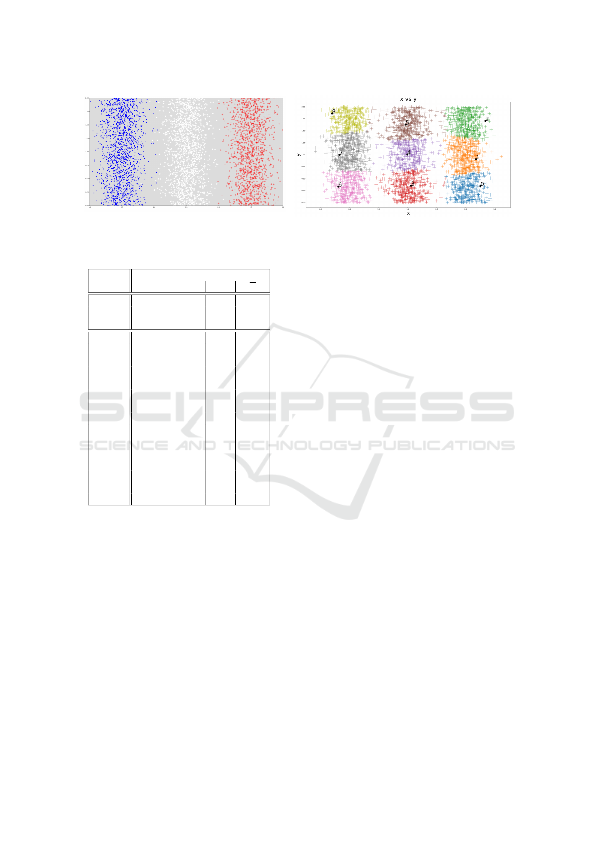
(a) The three distinct but slightly overlapping strips.

(b) The three strips projected onto a 3x3 grid.

Figure 1: The overlapping 2D-strips.

Table 1: Density and AvStd of the three 2D-strips.

Strips

Density

Standard deviation

dba0 407.44 0.17 0.59 0.38

dba1 388.88 0.18 0.58 0.38

dba2 403.13 0.17 0.58 0.38

clt0 534.39 0.17 0.18 0.17

clt1 463.67 0.16 0.22 0.19

clt2 503.95 0.16 0.19 0.18

clt3 382.01 0.19 0.20 0.19

clt4 378.72 0.19 0.18 0.19

clt5 347.15 0.22 0.20 0.21

clt6 507.68 0.16 0.19 0.18

clt7 539.01 0.17 0.23 0.20

clt8 531.27 0.15 0.15 0.15

Min 347.15 0.15 0.15 0.15

Max 539.01 0.22 0.23 0.21

Q1 382.01 0.16 0.18 0.18

Med 503.95 0.17 0.19 0.19

Q3 531.27 0.19 0.20 0.19

Mean 465.32 0.17 0.19 0.18

there is something weird with these three clusters.

It is what we were talking about in the above para-

graph: clusters #3, #4 and #5 overlap the others, what

makes them less dense. As all these clusters have a

similar shape, they should all have a similar density,

but the overlaps increase the density of the left and

right clusters and decrease that of the middle clusters.

This observation does not manifest itself with the

AvStd: 0.19, 0.19 and 0.21 for clusters #3, #4 and #5,

respectively. These values are slightly consistent with

those of the other clusters. This is due to the fact that

the outermost points, caught by the middle nodes, are

somehow outliers to them; the standard deviation is

little sensitive to outliers, reason of this consistency.

As a conclusion, through this example, the den-

sity measure has an advantage on the AvStd measure,

since it has allowed to point out the three overlapping

clusters, what the AvStd has not been able to do.

4.2 Gaussian Distributions

The second example is a set of Gaussian distributions,

in dimension n. We will start in dimension 3; then we

will move on to the greatly higher dimension 25 to

show the generalization capability of our metric.

4.2.1 Dimension 3

Let us start in dimension 3, with a set of twelve groups

of data, each generated with a Gaussian distribution.

The mean of any cluster is randomly drawn following

an uniform distribution within the feature space, rang-

ing from 0 to 10 units for each of the 3 dimensions.

Each 3D-Gaussian distribution contains 250 data in-

stances, with a standard deviation of 0.5 unit. Even

though this value is not prone to great overlaps, the

random drawing of the groups’ means makes possi-

ble and even probable some overlaps however.

This dataset mainly aims at showing the results

obtained within a 3-dimension feature space, and how

an overlap can be pointed out with our density mea-

sure, while not that easily with the AvStd measure.

The so-generated database is shown on Figure 2a

and the clustered database projected onto a (too small)

grid of size 3 × 3 is displayed on Figure 2b. The op-

position of any possible couple of dimensions



(x,y),

(x,z) and (y,z)



is represented as Figure 3, in order

to give a greater insight on the relations and overlaps

of the clusters, in any dimension. The results of the

quantifying measures are gathered within Table 2.

The ﬁrst thing is that several Gaussian distribu-

tions have been merged as a unique cluster, which is

not surprising, since the grid is too small (nine nodes

for twelve distributions): nodes #2, #3, #6 and #8 of

Figure 2b are such a merging. For some, this is not a

problem, since the groups are very close in the orig-

inal database: according to Figure 3, we can see that

cluster #3 is perfectly compact, and that its merging is

not a problem at all. But for the three remaining clus-

Characterizing N-Dimension Data Clusters: A Density-based Metric for Compactness and Homogeneity Evaluation

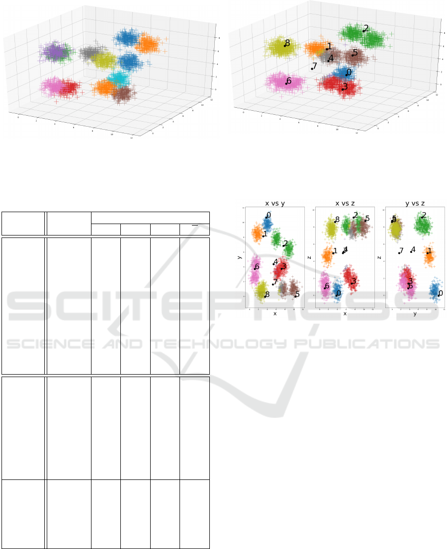
(a) The original 3D-Gaussian distributions, as random com-

pact groups of data, but with some local overlaps.

(b) The clustered 3D-Gaussian distributions, projected onto

a too small 3x3 grid, causing the merging or the splitting of

some groups whereas they should not be.

Figure 2: The 3D-Gaussian distributions.

Table 2: Density and AvStd of the twelve 3D-Gaussians.

Gauss

Density

Standard deviation

dba0 8.36 0.51 0.51 0.52 0.51

dba1 8.12 0.51 0.54 0.55 0.53

dba2 9.89 0.49 0.55 0.48 0.51

dba3 5.75 0.51 0.52 0.51 0.51

dba4 7.19 0.52 0.50 0.51 0.51

dba5 11.87 0.52 0.51 0.53 0.52

dba6 6.97 0.49 0.46 0.52 0.49

dba7 8.90 0.54 0.51 0.50 0.52

dba8 11.79 0.51 0.48 0.49 0.49

dba9 6.56 0.46 0.52 0.52 0.50

dba10 11.75 0.45 0.52 0.49 0.48

dba11 11.83 0.44 0.50 0.48 0.47

clt0 6.56 0.46 0.52 0.52 0.50

clt1 0.82 0.57 0.52 0.52 0.54

clt2 3.79 1.47 0.86 0.52 0.95

clt3 9.70 0.77 0.65 0.65 0.69

clt4 0.03 0.25 1.13 1.16 0.85

clt5 4.72 1.14 0.50 0.50 0.71

clt6 4.65 0.52 1.01 0.71 0.75

clt7 0.31 0.67 0.54 1.18 0.80

clt8 1.67 0.83 0.53 0.50 0.62

Min 0.03 0.25 0.50 0.50 0.50

Max 9.70 1.47 1.13 1.18 0.95

Q1 0.82 0.52 0.52 0.52 0.62

Med 3.79 0.67 0.54 0.52 0.71

Q3 4.72 0.83 0.86 0.71 0.80

Mean 3.58 0.74 0.70 0.70 0.71

ters, #2, #6 and #8, a gap between the original distri-

butions can be observed: the clusters are not compact.

This statement can also be drawn from Table 2:

”clt3” has the highest density (9.70 units, 46% greater

than the second highest value 6.56 units), meaning it

Figure 3: The 3D-Gaussian clusters projected onto any pos-

sible 2-dimension feature set.

is very compact; but this observation does not work

with the AvStd measure, since its value 0.69 is very

close to the mean 0.71. The density indicates here that

this cluster #3 is very well-built, since very compact,

whereas the AvStd says only to us that it is in the av-

erage, neither good nor bad. Nonetheless, our above

qualitative observations validate the density measure.

That is also true for clusters #2, #6 and #8: the

two ﬁrst have an average density, while the third has a

very poor one. For clusters #2 and #6, that is because

the two original Gaussian distributions are close from

each other, thus their merging is not really dreadful

(Figure 4). Cluster #8 has a very low density how-

ever, justiﬁed by a bad overlap with another cluster

(Figure 5). On the contrary, the AvStd measure indi-

cates that its average standard deviation is very good

– equal to the ﬁrst quantile. This is due to the fact that

cluster #8 has a little overlap, with few data belong-

ing to a very distinct – and distant – cluster. Since the

AvStd measure is lowly affected by outliers, its aver-

age standard deviation is very good, while its density

is not, since that one is severely affected by outliers.

What happens to cluster #8 is also true for cluster

IN4PL 2021 - 2nd International Conference on Innovative Intelligent Industrial Production and Logistics

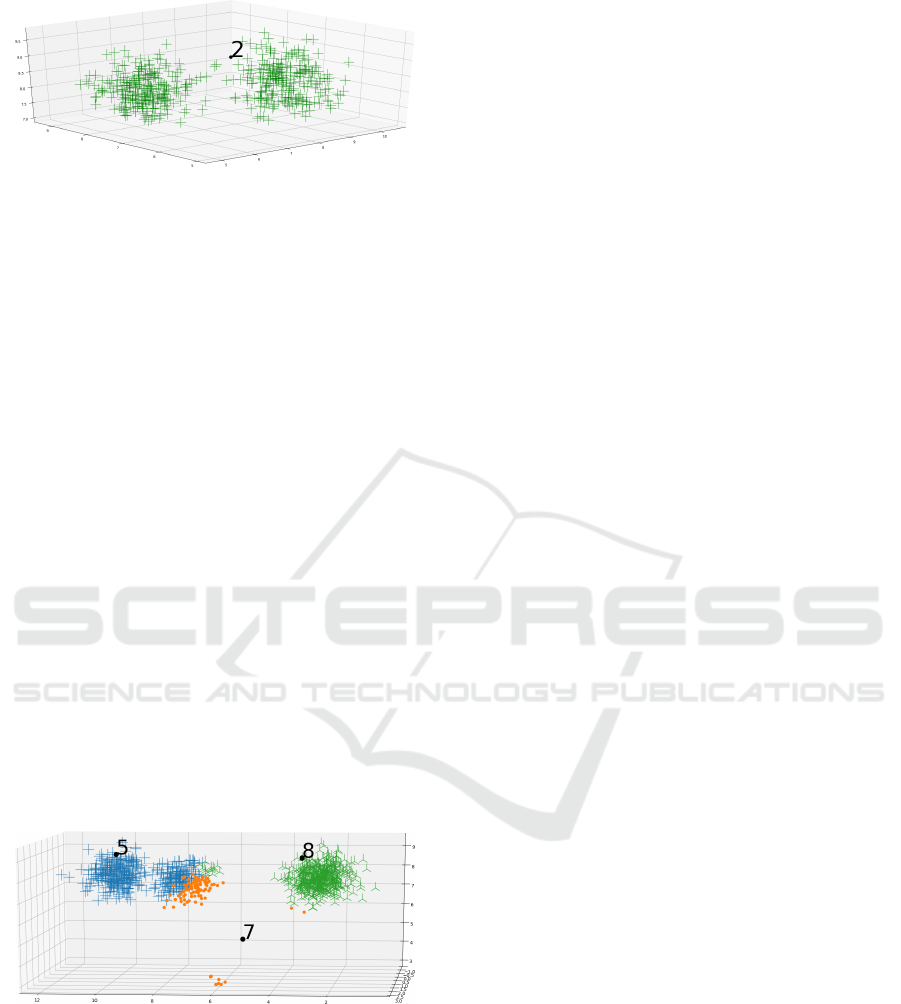
Figure 4: Zoom on cluster #2: it is not compact since it

gathers two independent, but near, distributions.

#1: it contains some distant outliers (should belong to

cluster #2), what greatly decreases its density.

The lowest density is achieved by cluster #4,

which contains very few data, dispatched within sev-

eral Gaussian distributions. This cluster is more an

outlier itself, what can be veriﬁed for its pattern is

nowhere, in between several clusters. Actually, it is

the middle node of the grid, reason why it ﬁnds itself

somehow in the middle of the feature space.

Finally, the last observation we can make is about

the two remaining clusters #5 and #7. A zoom on

them and on cluster #8 is displayed on Figure 5.

Indeed, these three clusters have some problems:

as already discussed, cluster #8 contains some out-

liers, what greatly decreases its density; cluster #5

overlaps another Gaussian distribution; and cluster #7

is alike #1: its pattern is nowhere, in the middle of the

ﬁgure, catching some points from here and there.

On Figure 5, one can notice that the Gaussian dis-

tribution right next to (the main part of) cluster #5 is

split into 3 sub-parts, one for each cluster among #5,

#7 and #8. Nonetheless, this distribution is very close

to cluster #5, as can be seen on Figure 3: a merging

of these two distributions is therefore not a big deal,

similarly to clusters #2 and #6.

Figure 5: Zoom on clusters #5, #7 and #8 as they all overlap

an independent, but unidentiﬁed, group. Note that cluster #7

overlaps 3 different clusters (middle bottom, middle right

and left), what causes it to have a very poor density, even

though its AvStd measure is perfectly acceptable.

All these observations can be understood from Ta-

ble 2 too: the density of clusters #7 and #8 are very

low, which means they are poorly compact. Unfor-

tunately, their AvStd, 0.8 and 0.62 respectively, are

anew in the average and acceptable compared to the

others: they do not really help to identify a possible

problem with these clusters, what their density, 0.31

and 1.67 respectively, did on the contrary.

As a conclusion, all our qualitative observations

have been validated by the density measure, and can

independently be made from them. This was rarely

the case with the AvStd measure, which is less af-

fected by outliers, but also less likely to point out

compactness and homogeneity troubles.

4.2.2 Dimension 25

Let’s now ﬁnish with a high dimension feature space.

The database is built following the same methodol-

ogy than that of section 4.2.1: twelve Gaussian distri-

butions, ranging from 0 to 10 in every dimension, a

standard deviation of 0.5 unit, with 250 points each,

but this time in dimension 25 instead of 3.

The purpose of such a database is to illustrate the

generalization capability of our metric, as blind users.

Indeed, as we are in a too highly dimensional feature

space for 2D or 3D representation, we will only give

quantitative avenues of reﬂection, without a real pos-

sibility to directly validate them through qualitative

observations. This represents a real blind – unsuper-

vised – evaluation for a Machine Learning application

within an Industry 4.0 context for instance.

Once more, the results obtained after clustering

are gathered within Table 3; ”None” entry represents

the absence of value, in case of the corresponding

cluster is empty (and might be pruned).

This example is interesting for is works on a per-

fect clustering of the database: any of the twelve

Gaussian distributions has been perfectly identiﬁed

and is represented by a unique node of the SOM’s

4 × 4 grid. One can be convinced of this by compar-

ing the ”dba” lines to the ”clt” lines: there is a perfect

correspondence for each, e.g. ”dba0” is ”clt4”.

So, what can we learn from this table? The mean

standard deviation, i.e. the AvStd measure, is consis-

tent within the twelve clusters, and is approximately

equal to 0.5 (which is coherent when compared to the

standard deviation used to generate the Gaussian dis-

tributions), thus the clusters seem coherent and com-

pact. This observation is also slightly true based on

the density measure, which is quite consistent too,

varying from 85.24 to 102.70 – an increase of 20.5 %.

The effective difference in the densities can be ex-

plained by the span of the clusters: even though they

share a very similar standard deviation, their outer-

most points are not all as distant from their respective

cluster’s mean. The density measure is sensitive to

that, what explains the small but real variation. As

such, in order to correctly use this measure, only very

Characterizing N-Dimension Data Clusters: A Density-based Metric for Compactness and Homogeneity Evaluation

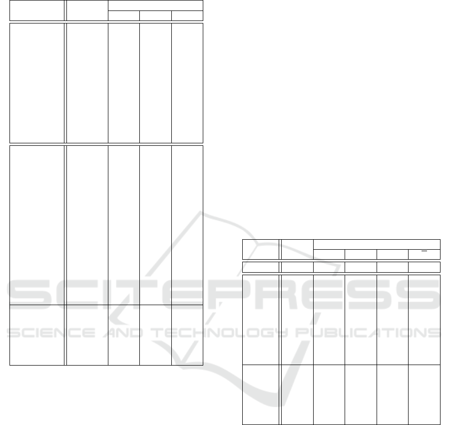
Table 3: Density and AvStd of the twelve 25D-Gaussians.

Gauss25

Density

Standard deviation

min mean max

dba0 102.70 0.46 0.50 0.53

dba1 97.07 0.45 0.49 0.52

dba2 95.98 0.47 0.50 0.54

dba3 92.12 0.47 0.50 0.54

dba4 85.24 0.46 0.50 0.56

dba5 99.00 0.46 0.50 0.54

dba6 99.28 0.47 0.50 0.55

dba7 94.34 0.46 0.50 0.55

dba8 94.68 0.47 0.50 0.54

dba9 97.75 0.43 0.50 0.54

dba10 88.45 0.45 0.49 0.53

dba11 94.64 0.47 0.50 0.56

clt0 94.34 0.46 0.50 0.55

clt1 95.98 0.47 0.50 0.54

clt2 94.64 0.47 0.50 0.56

clt3 99.28 0.47 0.50 0.55

clt4 102.70 0.46 0.50 0.53

clt5 None None None None

clt6 92.12 0.47 0.50 0.54

clt7 94.68 0.47 0.50 0.54

clt8 None None None None

clt9 None None None None

clt10 None None None None

clt11 88.45 0.45 0.49 0.53

clt12 99.00 0.46 0.50 0.54

clt13 97.75 0.43 0.50 0.54

clt14 97.07 0.45 0.49 0.52

clt15 85.24 0.46 0.50 0.56

Min 85.24 0.43 0.49 0.52

Max 102.70 0.47 0.50 0.56

Q1 93.78 0.46 0.50 0.54

Med 95.33 0.46 0.50 0.54

Q3 98.06 0.47 0.50 0.55

Mean 95.10 0.46 0.50 0.54

noticeable differences should be considered, that is to

mean higher than 20 % from min to max for instance.

Nonetheless, this variation could indicate a not so

compact cluster, which might be worth being split for

a higher homogeneity anyway. Unfortunately, this

conclusion strongly depends on the context and on the

data themselves: there is no real absolute answer, es-

pecially when using an unsupervised paradigm.

This example shows that the density measure is as

reliable as the AvStd in high dimensions, at least for

a perfect clustering. Added to the previous observa-

tions, it seems that our density measure is reliable to

both point out issuing clusters and qualify compact

clusters, in every dimension.

4.3 Industrial Data: Solvay Op

erations

Our last example is a real use-case, in order to validate

the relevancy of our metric on real Industry 4.0 data.

For conﬁdentiality concerns, we won’t explain in de-

tails how the Solvay Op

erations



’s plant works; we

will remain general, what is not a big deal, since we

want to study automatic knowledge extraction from

unsupervised Machine Learning-based clustering.

We let just the reader know that the plant fea-

tures hundreds of sensors, for many purposes; accord-

ing to the Solvay’s experts, some are more relevant

than the others. Indeed, during the production proce-

dure, some steps are essential, and a small local dis-

turbance can have a huge impact and totally disturb

the whole system. In the following, for representa-

tiveness concerns, only some of these most important

sensors are depicted. As such, the feature space is

the n-dimension Euclidean space represented by the

n most important sensors. We will limit ourselves to

only 3 sensors to be able to represent the results.

The raw 3D sensor’s data are represented on Fig-

ure 6a, and the clustered data on Figure 6b. The re-

sults are gathered within Table 4, and Figure 7 shows

any couple of dimensions to give a clearer insight on

the relation between the data and the clusters as well.

Table 4: Density and AvStd of the Solvay’s data.

Solvay Den.

Standard deviation

dba 4701 0.17 0.19 0.24 0.2

clt0 6290 0.01 0.01 0.10 0.04

clt1 2.7 0.03 0.00 0.05 0.03

clt2 None None None None None

clt3 1118 0.14 0.08 0.11 0.11

clt4 4.9 0.02 0.01 0.00 0.01

clt5 1.6 0.02 0.01 0.12 0.05

clt6 2948 0.04 0.10 0.11 0.08

clt7 137 0.03 0.02 0.05 0.03

clt8 2840 0.06 0.05 0.13 0.08

Min 1.6 0.01 0.00 0.00 0.01

Max 6290 0.14 0.10 0.13 0.11

Q1 4.3 0.02 0.01 0.05 0.03

Med 211 0.03 0.02 0.11 0.04

Q3 1576 0.04 0.06 0.11 0.08

Mean 1348 0.04 0.03 0.08 0.05

On Figure 6a and Figure 7, we can distinguish sev-

eral compact groups of data, from at least two and up

to perhaps four or ﬁve. This incertitude we have in

counting the clusters, even as human beings, is the

exact reason why a density, or similar, measure is es-

sential to understand the structure of the data. Indeed,

there are only 3 dimensions, and that is enough to dis-

seminate a doubt; imagine a hundred of dimensions:

for a human being, and even worse for a machine,

identifying the number of clusters is an impossible

task without an accurate and reliable criterion!

Howsoever, without taking into account the actu-

ally found clusters, Figure 7 displays 2 clusters for ”x

vs y”, 2 or 3 for ”x vs z”, and 2 or 3 too for ”y vs z”.

On Figure 6a, we can see 3, maybe 4, clusters: one

IN4PL 2021 - 2nd International Conference on Innovative Intelligent Industrial Production and Logistics

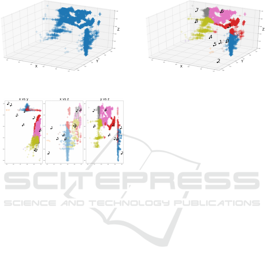
(a) The original 3D Solvay’s data.

(b) The 3D Solvay’s data projected onto a 3x3 grid.

Figure 6: Example of application on a real Industry 4.0 use-case: the Solvay’s data.

Figure 7: The Solvay’s clusters projected onto any possible

2-dimension feature set.

along Y-axis, one or two along Z-axis, and another

one along Y-axis anew, but shifted along X-axis.

The clustering method used is a 3 × 3 SOM, as

depicted on Figure 6b and Figure 7; ﬁve nodes seem

very large. Does this mean there are indeed 5 clusters

in the data? Let’s check this assumption out with the

results of Table 4.

Among all the nodes, cluster #2 is empty, and #1,

#4 and #5 have a poor density (they contain very few

data actually). The ﬁve remaining clusters, #0, #3, #6,

#7 and #8, have a small AvStd and a high density, ex-

cept #7, which is compact but contains some outliers.

Indeed, on Figure 6b and Figure 7, we can see

that these clusters are actually compact and accept-

able, except #3, which spans across clusters #0 and

#6. This cluster should be split, and its two parts

should be merged with these two clusters. This ob-

servation can also be drawn from Table 4: cluster #3

has the lowest density among the four valid, i.e. #0,

#3, #6 and #8, with a very noticeable gap, from 6290

units for the most dense to 1118 units for it – a de-

crease of 82%. Moreover, cluster #3 has the highest

AvStd, which means that its outermost data instances

are not outliers, but are real part of the cluster: that is

because it spans across two clusters.

Therefore, if we couple a low density with a high

AvStd, we can understand that cluster #3 has some

issues, and should be split to gain in homogeneity!

Cluster #0 is the only one to have a high density

and a very low AvStd, and can be trusted as represen-

tative of a local behavior of the system. Clusters #6

and #8 have a good density, but a quite high AvStd,

which means they are not real outliers, but they are

more likely spanning across several sub-regions of the

feature space: they might be worth being split!

As a conclusion, we have applied our density met-

ric on Industry 4.0 real data, and we have been able to

identify from 1 (sure) to 3 (very likely) and perhaps

4 (low probability) local behaviors. This short exam-

ple illustrates the potential of the density metric in a

real situation, that is to point out issuing clusters, es-

pecially when used alongside the AvStd measure (to

compensate its high sensitiveness to outliers).

Future Work. Now this metric is validated and

trustful, the next step of our work would be to apply

it on very wider databases related to Industry 4.0, in

order to extract knowledge by using data mining ap-

proaches, such as local behavior identiﬁcation. Once

done, the next step is to train a MES network, whose

neurons are local experts trained upon the data within

the identiﬁed local behaviors, and validated by a com-

pactness metric.

5 CONCLUSION

In this paper, we have introduced a compactness

density-based measure to quantify and validate the

quality of a n-dimension cluster.

This measure is computationally efﬁcient, since it

computes the cluster’s mean, searches for the farthest

point from it, and doubles this distance to obtain an

estimate of the cluster’s span. This value is then used

as the radius of a n-hyper-sphere, which is built to

contain all the data of the cluster, and to provide a n-

Characterizing N-Dimension Data Clusters: A Density-based Metric for Compactness and Homogeneity Evaluation

dimension boundaries estimate. Its volume is then as-

similated to that of the cluster. The density measure is

eventually deﬁned as the ratio of the number of points

contained within by that hyper-sphere’s volume.

We then compared and validated this measure to

a reference one, namely the Average Standard Devi-

ation AvStd. We applied both on several academical

datasets, before and after clustering, in order to show

the relevancy and the accuracy of both metrics. We

also studied the data provided by a real Industry 4.0

use-case – Solvay Op

erations



’s plant.

While the AvStd showed some good results, there

are several cases where it failed to identify an underly-

ing issue within the clusters, such as an almost empty

cluster or a small but real overlap of several clusters.

On the contrary, the density measure displayed

good results in both identifying clustering issues and

in indicating a cluster is compact and homogeneous.

Nonetheless, we also showed that the density mea-

sure is sensitive to outliers; that can be a problem for

some applications. This measure is therefore not per-

fect, and has its drawbacks. To better understand the

data, especially in a data mining context, one could

use both (or more) measures, namely AvStd and our

density measure, to qualify the clusters and evaluate

their compactness, how representative they are, etc.

Indeed, the AvStd measure indicates if a group of

data is centered around its mean, and is lowly sensi-

tive to outliers; the density is the reverse, since it in-

dicates if the group is compact, but is affected by out-

liers. A high density with a small AvStd means a very

compact group. A low density with a high AvStd indi-

cates scattered data. A high density with a high AvStd

means there are few outliers, but the data are scattered

nonetheless: it indicates a cluster is spanning across

several classes and thus not homogeneous.

Perhaps the best way to take beneﬁt from our met-

ric is to use it alongside some others, and to merge

their respective outputs. This trend is often true, since

there is no perfect method, especially with an unsu-

pervised Machine Learning-based approach like ours.

ACKNOWLEDGEMENTS

This paper takes place within the project Hypercon-

nected Architecture for High Cognitive Production

Plants HyperCOG, accepted on March 31

, 2020.

It has received funding from the European Union’s

Horizon 2020 research and innovation program un-

der grant agreement No 695965. Persistent identiﬁer:

HyperCOG -695965. Website: www.hypercog.eu.

REFERENCES

Boser, B., Guyon, I., and Vapnik, V. (1996). A training

algorithm for optimal margin classiﬁer. Proceedings

of the Fifth Annual ACM Workshop on Computational

Learning Theory, 5.

Broomhead, D. and Lowe, D. (1988). Radial basis

functions, multi-variable functional interpolation and

adaptive networks. Royal Signals and Radar Estab-

lishment Malvern (UK), RSRE-MEMO-4148.

Buchanan, B. and Feigenbaum, E. (1978). Dendral and

meta-dendral: Their applications dimension. Artiﬁcial

Intelligence, 11(1):5–24. Applications to the Sciences

and Medicine.

Davies, D. and Bouldin, D. (1979). A cluster separation

measure. Pattern Analysis and Machine Intelligence,

IEEE Transactions on, PAMI-1:224–227.

Dunn, J. (1974). Well-separated clusters and optimal fuzzy

partitions. Cybernetics and Systems, 4:95–104.

Dunn, J. C. (1973). A fuzzy relative of the isodata process

and its use in detecting compact well-separated clus-

ters. Journal of Cybernetics, 3(3):32–57.

Jain, A. K. (2010). Data clustering: 50 years beyond k-

means. Pattern Recognition Letters, 31(8):651–666.

Kohonen, T. (1982). Self-organized formation of topolog-

ically correct feature maps. Biological Cybernetics,

43(1):59–69.

Lawrence, A. E. (2001). The volume of an n-dimensional

hypersphere. University of Loughborough.

Martinetz, T. and Schulten, K. (1991). A ”neural-gas” net-

work learns topologies. Artiﬁcial neural networks,

1:397–402.

Rousseeuw, P. (1987). Silhouettes: A graphical aid to the in-

terpretation and validation of cluster analysis. Journal

of Computational and Applied Mathematics, 20:53–

65.

Rumelhart, D., Hinton, G., and Williams, R. (1986a).

Learning Internal Representations by Error Propaga-

tion, pages 318–362. MIT Press.

Rumelhart, D., McClelland, J., and PDP Research Group,

C., editors (1986b). Parallel Distributed Processing:

Explorations in the Microstructure of Cognition, Vol.

1: Foundations. MIT Press, Cambridge, MA, USA.

Russo, C. (2020). Knowledge design and conceptualiza-

tion in autonomous robotics. PhD thesis, Universities

Paris-Est XII, France and Naples Federico II, Italy.

Rybnik, M. (2004). Contribution to the modelling and the

exploitation of hybrid multiple neural networks sys-

tems : application to intelligent processing of infor-

mation. PhD thesis, University Paris-Est XII, France.

Shan, T. and Englot, B. (2018). Lego-loam: Lightweight

and ground-optimized lidar odometry and mapping

on variable terrain. In 2018 IEEE/RSJ International

Conference on Intelligent Robots and Systems, pages

4758–4765.

Thiaw, L. (2008). Identiﬁcation of non linear dynamical

system by neural networks and multiple models. PhD

thesis, University Paris-Est XII, France. (in French).

IN4PL 2021 - 2nd International Conference on Innovative Intelligent Industrial Production and Logistics