Lead Time Estimation of a Drilling Factory with Machine and Deep

Learning Algorithms: A Case Study

Alessandro Rizzuto

, David Govi

, Federico Schipani

and Alessandro Lazzeri

Deepclever S.r.l., Via Bure Vecchia Nord n.c. 115, 51100, Pistoia (PT), Italy

Keywords:

Lead Time, Machine Learning, Regression, Smart Manufacturing.

Abstract:

This project is presented as a real case-study based on machine learning and deep learning algorithms which

are compared for a clearer understanding of which procedure is more suitable to industrial drilling.The predic-

tions are obtained by using algorithms with a pre-processed dataset which was made available by the industry.

The losses of each algorithm together with the SHAP values are reported, in order to understand which features

most inﬂuenced the ﬁnal prediction.

1 INTRODUCTION

Dealing with production orders means adequately

managing a factory in order to satisfy the demand

generated by the customers. A factory manager could

gain huge beneﬁts by a forecasting system because it

can show alternative decisions that can be undertaken

in order to maintain an efﬁcient throughput via the

optimization of the available resources (Pfeiffer et al.,

2016). In order to face this challenge, many kinds

of diverse problems have arisen in the past decades:

some of them that are worth mentioning are predic-

tive maintenance, demand planning, scheduling and

lead time (LT) prediction (Cadavid et al., 2020). The

LT prediction is one of the most important elements

to keep in mind when one wants to properly face pro-

duction and planning control, since it can give hints

on how to distribute jobs among the available ma-

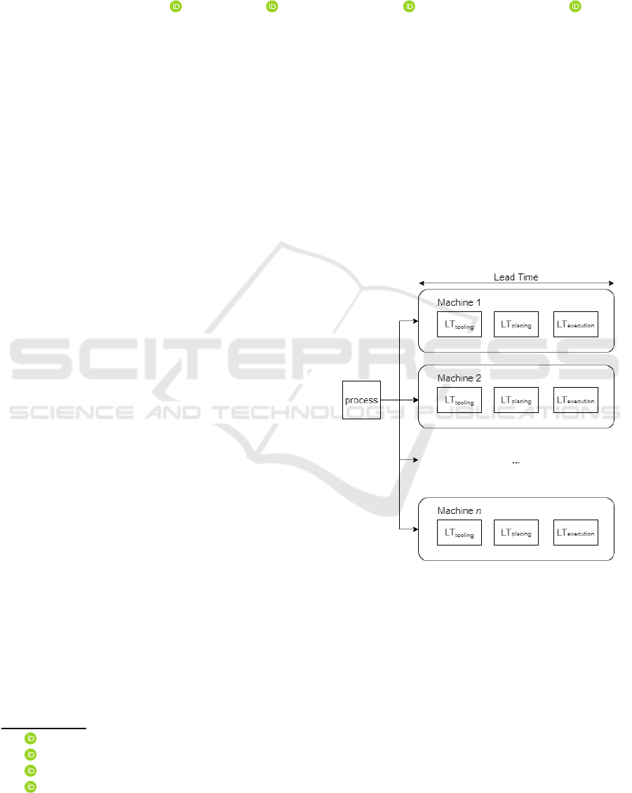
chines. For example, in Figure 1, the drilling machine

has three process steps: the tooling time, representing

the time required for preparing a resource; the plac-

ing time, namely the time that has to be employed to

place an object in a machine correctly; the execution

time, describing how many minutes are necessary to

drill the object. The more accurate are the estimations

of the lead time of a process on the machines, the bet-

ter the productionmanager can schedule the processes

and meet the customers needs. However, most of

https://orcid.org/0000-0002-1074-1035

https://orcid.org/0000-0001-6283-3225

https://orcid.org/0000-0002-6119-7033

https://orcid.org/0000-0003-3112-9010

Figure 1: Illustration of Lead Time analysis.

the research has focused mostly on data mining pro-

cedures and has exploited datasets created thanks to

discrete event simulation (Lingitz et al., 2018) (Pfeif-

fer et al., 2016): this is a great limit to the predictive

power of an algorithm, since the usage of well-known

events could bring to the exclusion of several other

factors that could impact the ﬁnal time value that has

to be employed in order to complete a process. In-

stead, the adoption of Machine Learning procedures

can trigger the discovery of patterns hidden inside the

data, allowing to link features that were previously ex-

cluded from the analysis of the problem (Lingitz et al.,

Rizzuto, A., Govi, D., Schipani, F. and Lazzeri, A.

Lead Time Estimation of a Drilling Factory with Machine and Deep Learning Algorithms: A Case Study.

DOI: 10.5220/0010655000003062

In Proceedings of the 2nd International Conference on Innovative Intelligent Industrial Production and Logistics (IN4PL 2021), pages 84-92

ISBN: 978-989-758-535-7

2018). For an in-depth study, it was decided to exam-

ine the feature importance of the Machine Learning

techniques, but these values are not completely reli-

able when several different models have to be eval-

uated: indeed importance is biased over the charac-

teristic of the model taken into consideration (Lund-

berg and Lee, 2017). Thus, it was decided to exploit

SHAP (i.e.: SHapley Additive exPlanations) which

implements an additivestrategy for measuring the real

impact of each single feature to the predicted value:

this is possible thanks to an approach derived from

the game theory, through the average of the marginal

contribution of all the possible feature permutations

(Lundberg and Lee, 2017).

1.1 Related Works

Lingitz et. al. (Lingitz et al., 2018) studied the case

of a semiconductor manufacturing process by apply-

ing a series of Machine Learning algorithms, consist-

ing of several linear regressors, an ensemble of deci-

sion trees, support vector machines and artiﬁcial neu-

ral networks. The authors did not evaluate gradient-

boosted decision trees which are adopted nowadays in

several regression tasks (Chen and Guestrin, 2016).

Pfeiffer et. al. (Pfeiffer et al., 2016) developing a

discrete event simulator which allows a reliable de-

scription of the factory, then they trained some Ma-

chine Learning models, showing that random forests

are able to overcome linear regression and regression

trees in terms of performances. In this work, the il-

lustrated algorithms are bound to the discrete event

generation. Gyulai et. al. (Gyulai et al., 2018) made a

comparison between analytical and Machine Learn-

ing techniques by exploiting a job-shop which un-

derwent several changes. This work focuses only on

three supervised learning approaches, which are lin-

ear regression, support vector and tree-based mod-

els. Onaran et. al. (Onaran and Yanik, 2019) took

data from a textile manufacturingsystem and trained a

neural network in order to estimate the necessary time

for planning the jobs. This work focuses on a certain

industry, that is, the textile one: this suggests that for

each domain it is necessary to gain the appropriate

knowledge for investigating how the features impact

on a learning model and which algorithm better ﬁts

the task. Indeed, the model and feature selection is

strongly dependent on the production environment of

interest, therefore there is no rule to choose an algo-

rithm but it is necessary to perform a deep study of

the industry of interest (Gyulai et al., 2018).

1.2 Contribution and Novelty

The main contributions of this paper are:

• the analysis of the features of three important pro-

cessing times of drilling operations;

• the application and comparison of several ML al-

gorithms to predict the processing times;

• the evaluation of the features with SHAP.

The paper is structured as follows: Section 2 pro-

vides the formal statement of the problem. Section

3 illustrates the state-of-the-art ML implemented al-

gorithms. Section 4 summarizes the adopted settings

for each single ML algorithm, together with the ﬁnal

results derived by the experiments. Finally, conclu-

sions are discussed and future works are described in

Section 5.

2 PROBLEM STATEMENT

Each job j comes from a set J, that is: j ∈ J with

J = {1,2,... ,m}. A job is characterized by a series

of processes p ∈ P with P = {1,2,..., n} that has to

be completed (in this case, n = 3). The machine u ∈ U

with U = {1, 2,. .., q} is the processing unit which

performs a process. The completion of a process em-

ploys a speciﬁc amount of time t, depending on the

couple process-machine hp,ui. The vector x ∈ R

of features describes the process p, thus the LT pre-

diction problem can be formulated as follows: given

the features x that distinguish the process p coming

from P, there is interest in ﬁnding a function

f, able

to retrieve t

∗

∈ R, which is the predicted time value

that has to be the nearest as possible to the true value

t ∈ R described by its corresponding target function

f. It is desirable to retrieve a function

f which re-

ports the smallest possible error with respect to the

outputs given by the original f:

E =

∑

( f(x) −

f(x))

(1)

In this way, the correct weights that will be assigned

to the approximated function

f can be determined

(Mitchell, 1997). In order to perform this task efﬁ-

ciently, a proper evaluation metric must be selected to

achieve an accurate error measurement between the

original and predicted values. Therefore, RMSE (i.e.:

Root Mean Squared Error) was exploited:

RMSE =





∑

i=1

− t

∗

)

(2)

The RMSE gives a higher penalty the more a sam-

ple differs from the mean and it is more suitable when

the errors follow a Gaussian distribution.

Lead Time Estimation of a Drilling Factory with Machine and Deep Learning Algorithms: A Case Study

On the other hand, the MAE (i.e.: Mean Absolute

Error)

MAE =





∑

i=1

− t

∗

| (3)

is easier to interpret, despite assigning to the samples

the same weight: hence, it is a good measurement of

the bias inherent in the model (Tianfeng and Draxler,

2014). Finally, it is supposed that the time t only de-

pends on the couple hp,ui, thus some assumptions

were made about the dataset: ﬁrst, it is supposed that

all the machines reported are the only ones that are

able to perform that speciﬁc drilling operation. Sec-

ondly, all the machines are located in the same in-

dustry, without further logistical distinctions. Lastly,

no machine suffered a blackout or any other adverse

event: this brings to the supposition that all the ma-

chines remained in the same state during the comple-

tion of the processes.

3 PREDICTING LEAD TIME

WITH ML ALGORITHMS

Several Machine learning methods have been evalu-

ated for the LT prediction. Among them, it is possi-

ble to distinguish ﬁve families of algorithms: Linear

models, Ensemble Tree methods, Gradient-Boosted

Decision Trees (i.e.: GBDT) and Neural Networks

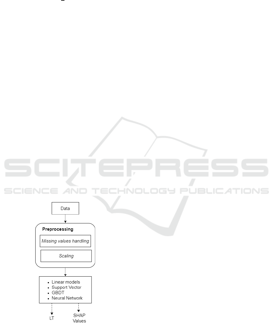
(i.e.: NN). Before proceeding, the pipeline that the

data has undergone will be illustrated.

Figure 2: Data pipeline.

The main reason is to understand the most promis-

ing procedures that can discover those relations which

can bring to a more accurate prediction of how long

a drilling process will take, given the data. This task

is crucial in order for and industry to perform the best

production planning, and it is a rising research ﬁeld in

the manufacturing domain (Lingitz et al., 2018).

3.1 Linear Models

Linear models are based on ﬁnding the relationships

occurring among independent variables with respect

to a target, independent variable (Gyulai et al., 2018).

To reach this goal, linear models have to minimize an

empirical loss which contributes to the retrieval of the

coefﬁcients of a function (Russell and Norvig, 2009).

The basic linear regression approach is based on re-

ducing the residual sum of squares, while more com-

plex methods such as Ridge and Lasso apply a regu-

larization step, by exploiting L1 (i.e.: the Mean Ab-

solute Error) and L2 (i.e.: the Mean Squared Error)

penalty respectively.

3.2 Ensemble Tree Methods

An ensembling method, as the name suggests, con-

sists in combining a series of learning techniques,

such as Decision Trees, to improve the overall per-

formances. The idea is that putting together ”weaker”

structures allows to obtain a stronger and more pre-

cise predictor. A Bagging regressor is an ensembling

method which consists in training each single classi-

ﬁer on portion of random samples from the training

set, while Boosting uses a series of structures in order

to improve the performance of a learner on the basis

of what happened previously along the chain (Opitz

and Maclin, 1999). Random Forest can be seen as

a Bagging method with a further step: in addition to

train different decision trees by sampling the training

set, this methodology employs a random selection of

features (Ho, 1995).

3.3 Gradient-boosted Decision Trees

GBDT (i.e.: Gradient-Boosted Decision Tree) is a

family of algorithm that employs a gradient descent

procedure for improving predictions. The gradient

learning phase allows to identify structures that will

be added subsequently to the set of weak learners: in-

tuitively, the regressor underwent a phase called ad-

ditive step. That is: GBDT exploits decision trees

which are improved by updating the parameters re-

sponsible for the splits in each node, through the im-

plementation of an additive strategy (Si et al., 2017).

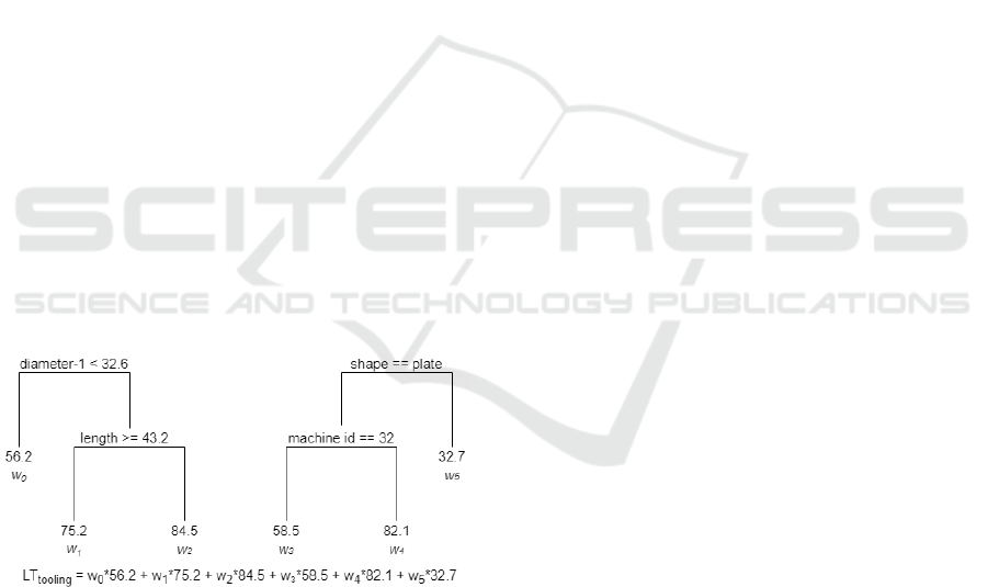
A simple example of how GBDT works is shown in

Figure 3. Over the last few years, two GBDT al-

gorithms stood out for their efﬁciency on real-world

IN4PL 2021 - 2nd International Conference on Innovative Intelligent Industrial Production and Logistics

datasets: XGBoost (i.e.: eXtreme Gradient Boosting)

(Chen and Guestrin, 2016) and Catboost (i.e.: Cate-

gorical Boosting) (Prokhorenkova et al., 2018). XG-

Boost is a a highly efﬁcient GBDT algorithm which

is often implemented in Kaggle challenges and it rep-

resents the state-of-the-art in many standard classiﬁ-

cation benchmarks (Chen and Guestrin, 2016). It fol-

lows the same idea behind Gradient-Boosting algo-

rithms, with minor improvements. The strong point

of the XGBoost is that it lies on the speed of execu-

tion and computational efﬁciency: as a matter of fact,

it properly faces the problem of sparsity in datasets

and implements a column block strategy for parallel

computing (Chen and Guestrin, 2016). Catboost tack-

les an important problem: the authors underline the

presence of a statistical issue when categorical fea-

tures are dealt with. This issue is called conditional

shift and is caused by the difference among the dis-

tributions characterizing each single feature with re-

spect to the target value (Prokhorenkovaet al., 2018).

The solution proposed is based on the ordering princi-

ple, hence the name ordered TS: the training samples

are taken sequentially, thanks to the introduction of

an artiﬁcial ”time”. Even the boosting phase relies on

the aforementioned strategy, and it is called ordered

boosting: this procedure is based on the usage of ran-

dom permutations of the training set, in order to eval-

uate the splits generated by the tree structure. Ad-

ditionally, Catboost implements the combinations of

categorical features as new categorical features in or-

der to intercept hidden dependencies among the data

(Prokhorenkova et al., 2018).

Figure 3: Brief illustration of how GBDT works.

3.4 Neural Network

Neural Networks, also known as Multi-Layer Percep-

trons, are deep learning-based models resulting in

groundbreaking breakthroughs over the last decade,

since they enabled high performance achievement in

many different tasks (Wang et al., 2017). The name

MLP derives by the presence of neurons, or percep-

trons, which are in charge of sending the signal to the

other neurons placed in the following layer. The sig-

nal is sent when a threshold value is overcome: the

neurons have to compute an activation function in or-

der to send the output to the subsequent perceptrons.

This approach resembles how neurons send their sig-

nal to the others inside the human brain (Goodfellow

et al., 2016). The training phase of these complex

structures is constituted by a forward and a backward

propagation: once the network was fed with values

in a forward direction, the backward step optimizes

the weights, in order to improve the accuracy of the

model. Moreover, backward propagation allows to

perform the gradient descent, thus being crucial for

the learning phase (Goodfellowet al., 2016). Through

the application of the appropriated activation func-

tions, a neural network can perform smoothly a re-

gression task: as a matter of fact, linear activation

functions allow to outline a deep model able to pre-

dict continuous values (Goodfellow et al., 2016).

4 EXPERIMENTAL SETTING

The comparisons among algorithms were performed

by exploiting the dataset provided by the factory and

having the structure depicted in Table 1. For each tar-

get time, such as tooling, placing, and execution, a

speciﬁc regressor has been trained. Due to the pres-

ence of several misleading time and missing values,

a deep preprocessing study was conducted in order to

remove those records being at the extremes of each

single feature distribution. Hence, the missing val-

ues were treated as follows: in the case of num-

bers, a symbolic −1 was placed in order to make a

distinction between the absence of any value and 0,

while an

unknown

keyword is used in order to iden-

tify the lack of category. Moreover, both the features

and the target time have been standardized according

to: z = (x − µ)/σ. Finally, the categorical features

have been encoded in binary features; this last step is

not needed for the Catboost algorithm which requires

intact categorical features, since the algorithm takes

charge of their transformation into more informative

features (Prokhorenkova et al., 2018). The validation

was performed on the entire dataset by implement-

ing a 10-fold cross-validation: that is, the data un-

derwent k times (in this case, 10 times) a validation

phase, each time using a different partition. Then,

the resulting metrics are averaged out across the folds

(Mitchell, 1997). 10-fold cross validation allows to

obtain a reliable estimate of the classiﬁers, especially

in the case when one has to deal with a limited num-

ber of samples (Mitchell, 1997).

Lead Time Estimation of a Drilling Factory with Machine and Deep Learning Algorithms: A Case Study

Table 1: Description of the dataset.

Feature Original name Type Values Description

machine id id macchina C (object) 3-109 identiﬁer of the machine

# of objects n.pezzi N (int) 1-14 objects drilled in that job

# of holes

n fori N (int) 1-4 number of holes in that job

diameter Ø N (ﬂoat) 3-100 diameter of cylindrical object

depth

profond N (ﬂoat) 85-2290 cm to be drilled

shape forma C (object) [cylinder, square, shape of the object

plate]

through-hole passante B (int) [0, 1] through-hole or not

diameter-1

Ø-1 N (ﬂoat) 25-440 diameter of ﬁrst drill

diameter-2 Ø-2 N (ﬂoat) 25-280 diameter of second drilling

length

lungh N (ﬂoat) 188-5065 length of the object

material materiale C (object) [c40, k100, aisi, material of the object

alrmbr, 3062, steel]

C means Categorical feature, N stands for Numerical feature and B identiﬁes a Booelean feature

Table 2: Results for tooling time target value.

RMSE mean RMSE std MAE mean MAE std

Ridge 0.6817 0.2662 0.4804 0.1517

Lasso 0.7 0.2916 0.4983 0.1533

Random Forest

0.5934 0.3337 0.3873 0.1846

Bagging 0.6443 0.3352 0.4148 0.1951

SVR (linear kernel)

0.6914 0.34 0.4233 0.197

SVR (rbf kernel) 0.6627 0.2587 0.4214 0.1875

LGBM

0.7104 0.3415 0.5012 0.1433

XGB 0.6504 0.3415 0.3787 0.1862

Catboost

0.6093 0.1764 0.4437 0.1124

MLP (single) 0.6872 0.3081 0.4296 0.1605

MLP (multi)

0.6114 0.0723 0.4038 0.0353

4.1 Evaluation of the Models

The following models were built through the usage

of the

sci-kit

package: Ridge and Lasso Regres-

sion, Random Forest, Bagging, Support Vector Re-

gressor with linear and polynomial kernels, LGBM

(i.e.: Light Gradient Boosting Machine) regressor.

These models were implemented using the default pa-

rameters, with the exception of the linear models, hav-

ing a value of ﬁt intercept set to

False

, due to the

previous standardization of the dataset. The other pa-

rameters are the following: Random Forest regressor

uses 100 estimators with a minimum samples split of

2; Bagging regressor employs 10 estimators; Linear

SVR uses a linear kernel with a tolerance of 1e

−4

and a regularization parameter of 1, while SVR im-

plements an rbf (i.e.: Radial Basis Function) kernel,

a tolerance equals to 1e

−3

, a regularization parameter

of 1 and a ε value of 0.1; LGBM regressor was im-

plemented with a GBDT learning algorithm, a learn-

ing rate of 0.1, a number of estimators equals to 100

and with a maximum number of 31 leaves; XGB re-

gressor comes with a learning rate of 0.3, a maxi-

mum depth of the learner equals to 6 and 100 esti-

mators. Scikit is a high-level library that allows to

exploit many Machine Learning techniques with ease

of use and it represents the state-of-the-art for Python

developers (Pedregosa et al., 2012). Catboost regres-

sors were instantiated thanks to the ofﬁcial

Catboost

library (Prokhorenkova et al., 2018), with the follow-

ing parameters: a number of iterations equals to 200,

a maximum of depth of each single tree set to 6, to-

gether with a maximum number of leaves of 64 and a

learning rate of 0.09. The cost function employed for

the Catboost regressors training phase was the RMSE

(see equation 2). The four neural networks were de-

signed through the usage of the PyTorch library. Py-

Torch has become one of the most popular libraries

in the deep learning ﬁeld: the main reasons reside on

its ﬂexibility, being truly Pythonic thanks to its syn-

tax and its leverage of CUDA library to support GPU

hardware acceleration (Paszke et al., 2019). The fol-

lowing hyper-parameters were assigned to the neural

networks: weight decay equals to 1e

−3

, learning rate

IN4PL 2021 - 2nd International Conference on Innovative Intelligent Industrial Production and Logistics

Table 3: Results for placing time target value.

RMSE mean RMSE std MAE mean MAE std

Ridge 0.6378 0.1392 0.449 0.0841

Lasso 0.6487 0.1338 0.4653 0.0673

Random Forest

0.6311 0.1845 0.4042 0.1296

Bagging 0.6692 0.1727 0.4294 0.1321

SVR (linear kernel)

0.6699 0.1675 0.4596 0.1127

SVR (rbf kernel) 0.6128 0.1306 0.408 0.097

LGBM

0.6607 0.1014 0.49 0.084

XGB 0.6504 0.192 0.3737 0.15

Catboost

0.5565 0.1012 0.4111 0.0774

MLP (single) 0.6243 0.1954 0.4153 0.1262

MLP (multi)

0.6213 0.0674 0.4033 0.058

Table 4: Results for execution time target value.

RMSE mean RMSE std MAE mean MAE std

Ridge 0.85 0.3658 0.5449 0.216

Lasso 0.873 0.326 0.6061 0.164

Random Forest

0.6259 0.3121 0.3632 0.1415

Bagging 0.6567 0.31 0.3746 0.1535

SVR (linear kernel) 0.8603 0.3606 0.473 0.1931

SVR (rbf kernel)

0.6777 0.2616 0.4042 0.1323

LGBM 0.6211 0.2051 0.4257 0.109

XGB

0.5924 0.3307 0.3273 0.1541

Catboost 0.5831 0.1842 0.3907 0.0839

MLP (single)

0.708 0.2268 0.4535 0.1076

MLP (multi) 0.6494 0.1165 0.3985 0.0663

set to 1e

−3

, batch size set to 64. After testing sev-

eral networks, it was decided to adopt the following

layer-wise structure:

input

→

[

64, 128, 64, 32] →

output

. In the case of target-wise neural networks,

output

is equal to 1, while for the multiple outputs

architecture

output

is set to 3 (i.e.: the total num-

ber of target values). The

input

value is 50 due to

the columns expansion caused by the new dummy

columns generated by the preprocessing phase. Ta-

bles 2, 3 and 4 illustrate the RMSE and MAE metrics

with respect to the target values (i.e.: tooling, placing

and execution), together with the standard deviation.

4.2 Results and Discussions

The results show that tree-based methods outperform

linear models and complex architectures: this is in

line with other applications of the Random Forest

within the manufacturing ﬁeld (Pfeiffer et al., 2016)

(Lingitz et al., 2018) (Gyulai et al., 2018). However,

the resulting Catboost metrics are promising too: the

RMSE value overcame the one returned by Random

Forest in the case of placing and execution. Figures 4,

5 and 8 represent the SHAP values for Catboost, Ran-

dom Forest and multi-output Neural Network regres-

sors, respectively. Catboost retrieves some interesting

patterns by exploiting the potential of the categorical

features combination: indeed, machine id and shape

are some of the most informative characteristics and

allow an estimate of the LT of a process on the ba-

sis of the ID number of a resource, together with the

shape of the object. On the other hand, Random For-

est underlines the importance of # of objects: the more

the number of objects to be processed, the more the

predicted time value. Continuous features are privi-

leged, even though the shape plate and the machines

numbered 31 and 32 have an important impact on the

model. Multi-output NN returns high SHAP values

for features that had a lower inﬂuence in the tree-

based models. Figures 6 and 7 depict several decision

functions that are plot against each single target value

together with the feature that correlates the most (i.e.:

diameter-1). Due to the fact that this was the ﬁrst time

that this industry collects data, there was no chance of

comparing the efﬁciency of the factory prior to this

study.

Lead Time Estimation of a Drilling Factory with Machine and Deep Learning Algorithms: A Case Study

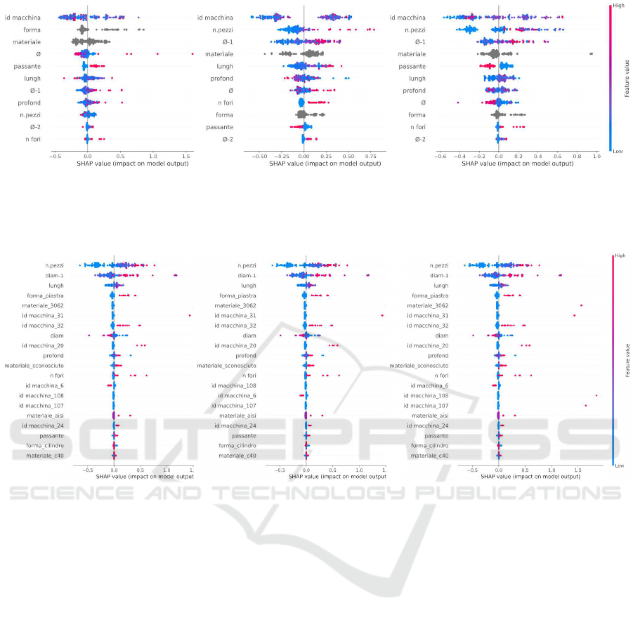
(a) SHAP values for tooling (b) SHAP values for placement (c) SHAP values for execution

Figure 4: SHAP values when Catboost is used. The blobs help to ﬁnd those values which inﬂuence the ﬁnal predicted value

the most. The color indicates whether the blobs contain lower or higher values. Each sub-ﬁgure depicts the impact of the

features for each single target variable.

(a) SHAP values for tooling (b) SHAP values for placement (c) SHAP values for execution

Figure 5: SHAP values when Random Forest is used. The blobs help to ﬁnd those values which inﬂuence the ﬁnal predicted

value the most. The color indicates whether the blobs contain lower or higher values. Each sub-ﬁgure depicts the impact of

the features for each single target variable.

5 CONCLUSIONS AND FUTURE

WORKS

This study compares several Machine Learning al-

gorithms in order to determine which one is the

most promising in terms of LT prediction in factory

drilling. The results of the experiment show that tree-

based methods outperform linear models and deep ar-

chitectures. The implementation of such automated

systems can bring huge beneﬁts for all those mecha-

nisms that regard decision making. Furthermore, the

analysis of the SHAP values bring out which features

impact the ﬁnal predicted value the most, enabling

further investigations on which parameters have to be

involved in forecasting Lead Time of a speciﬁc indus-

try. Although repeating the experiment on other in-

dustries will be necessary, the proposed method helps

to identify the best features for the prediction task.

This will reduce the effort of industries in collecting

data and install sensors on their equipment, stimulat-

ing the adoption of Machine Learning based systems.

Therefore, a further step of the research would be ex-

tending this kind of experimentation to other manu-

facturing industries, keeping an eye on GBDT, since

they resulted in being the most promising ones in

terms of Lead Time prediction.

ACKNOWLEDGMENTS

We thank the anonymous reviewers for their construc-

tive feedback and Simone Giovannetti for proofread-

ing the article. We wish to thank Polaris Engineering

S.r.l. for ﬁnancially supporting this research as well

as providing invaluable technical knowledge.

IN4PL 2021 - 2nd International Conference on Innovative Intelligent Industrial Production and Logistics

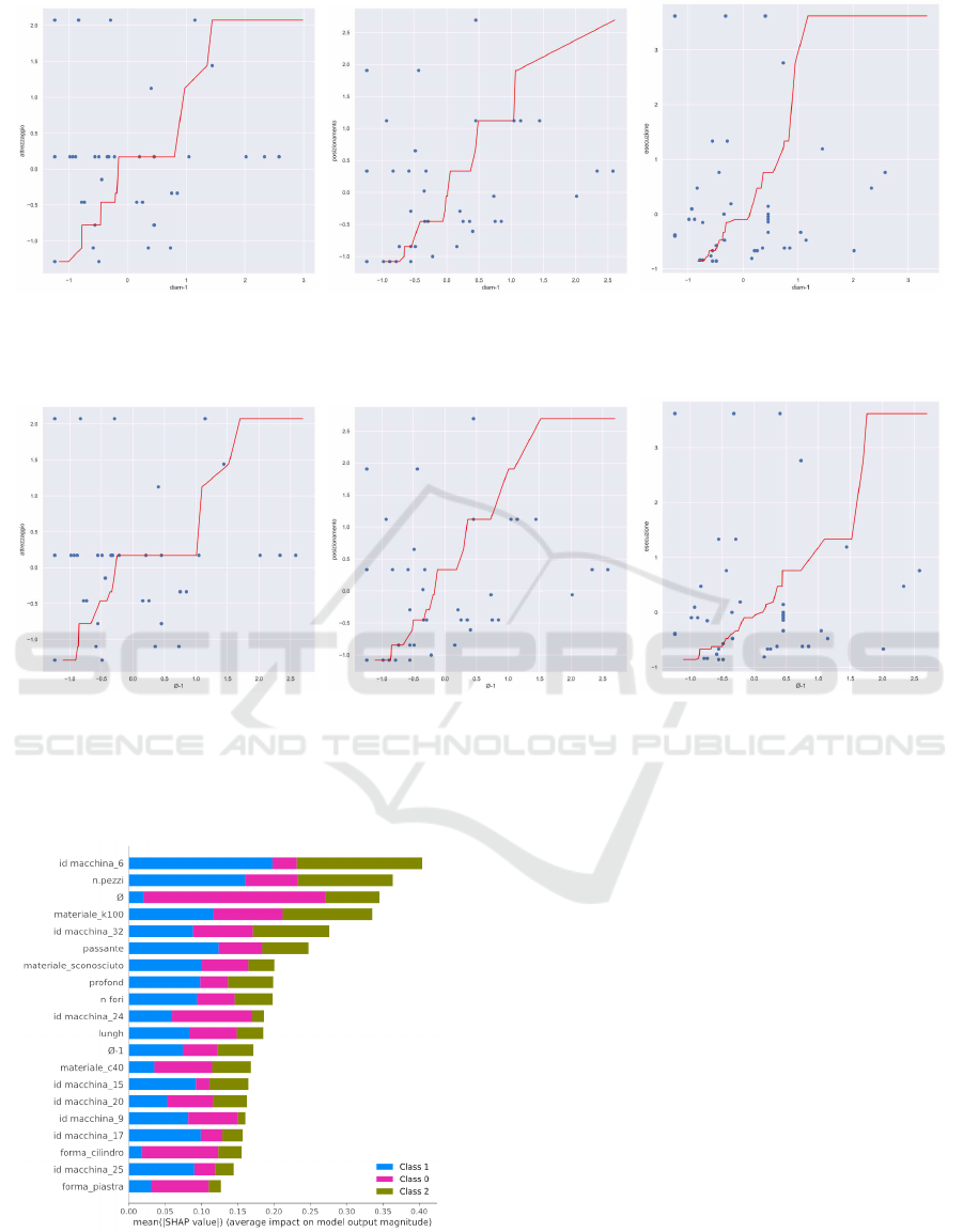
(a) SHAP values for tooling (b) SHAP values for placement (c) SHAP values for execution

Figure 6: Plot of the decision function in Random Forest. For a 2-dimensional plot, each target variable is represented together

with the feature diameter-1, which is one of the features that correlates the most.

(a) SHAP values for tooling (b) SHAP values for placement (c) SHAP values for execution

Figure 7: Plot of the decision function in Catboost. For a 2-dimensional plot, each target variable is represented together with

the feature diameter-1, which is one of the features that correlates the most.

Figure 8: Average impact of SHAP values for each target

variable when using multiple-outputs Neural Network.

REFERENCES

Cadavid, U., Pablo, J., Lamouri, S., Grabot, B., Pellerin, R.,

and Fortin, A. (2020). Machine learning applied in

production planning and control: a state-of-the-art in

the era of industry 4.0. Journal of Intelligent Manu-

facturing, 31.

Chen, T. and Guestrin, C. (2016). Xgboost: A scalable

tree boosting system. In Proceedings of the 22nd

ACM SIGKDD International Conference on Knowl-

edge Discovery and Data Mining. Association for

Computing Machinery.

Goodfellow, I., Bengio, Y., and Courville, A. (2016). Deep

Learning. The MIT Press.

Gyulai, D., Pfeiffer, A., Nick, G., Gallina, V., Sihn, W.,

and Monostori, L. (2018). Lead time prediction in

a ﬂow-shop environment with analytical and machine

learning approaches. IFAC-PapersOnLine. 16th IFAC

Symposium on Information Control Problems in Man-

ufacturing INCOM 2018.

Ho, T. K. (1995). Random decision forests. In Proceedings

of the Third International Conference on Document

Lead Time Estimation of a Drilling Factory with Machine and Deep Learning Algorithms: A Case Study

Analysis and Recognition (Volume 1) - Volume 1, IC-

DAR ’95, USA. IEEE Computer Society.

Lingitz, L., Gallina, V., Ansari, F., Gyulai, D., Pfeiffer, A.,

Sihn, W., and Monostori, L. (2018). Lead time predic-

tion using machine learning algorithms: A case study

by a semiconductor manufacturer. Procedia CIRP.

51st CIRP Conference on Manufacturing Systems.

Lundberg, S. and Lee, S.-I. (2017). A uniﬁed approach to

interpreting model predictions. In Guyon, I., Luxburg,

U. V., Bengio, S., Wallach, H., Fergus, R., Vish-

wanathan, S., and Garnett, R., editors, Advances in

Neural Information Processing Systems. Curran As-

sociates, Inc.

Mitchell, T. (1997). Machine Learning. McGraw Hill Inc.,

USA, 1st edition.

Onaran, E. and Yanik, S. (2019). Predicting Cycle Times

in Textile Manufacturing Using Artiﬁcial Neural Net-

work.

Opitz, D. and Maclin, R. (1999). Popular ensemble meth-

ods: An empirical study. Journal of Artiﬁcial Intelli-

gence Research.

Paszke, A., Gross, S., Massa, F., Lerer, A., Bradbury,

J., Chanan, G., Killeen, T., Lin, Z., Gimelshein,

N., Antiga, L., Desmaison, A., K¨opf, A., Yang, E.,

DeVito, Z., Raison, M., Tejani, A., Chilamkurthy,

S., Steiner, B., Fang, L., Bai, J., and Chintala, S.

(2019). In Wallach, H., Larochelle, H., Beygelzimer,

A., d'Alch´e-Buc, F., Fox, E., and Garnett, R., editors,

Advances in Neural Information Processing Systems,

volume 32. Curran Associates, Inc.

Pedregosa, F., Varoquaux, G., Gramfort, A., Michel, V.,

Thirion, B., Grisel, O., Blondel, M., Prettenhofer, P.,

Weiss, R., Dubourg, V., Vanderplas, J., Passos, A.,

Cournapeau, D., Brucher, M., Perrot, M., Duchesnay,

E., and Louppe, G. (2012). Scikit-learn: Machine

learning in python. Journal of Machine Learning Re-

search, 12.

Pfeiffer, A., Gyulai, D., K´ad´ar, B., and Monostori, L.

(2016). Manufacturing lead time estimation with

the combination of simulation and statistical learning

methods. Procedia CIRP.

Prokhorenkova, L., Gusev, G., Vorobev, A., Dorogush,

A. V., and Gulin, A. (2018). Catboost: Unbiased

boosting with categorical features. In Proceedings of

the 32nd International Conference on Neural Infor-

mation Processing Systems. Curran Associates Inc.

Russell, S. and Norvig, P. (2009). Artiﬁcial Intelligence:

A Modern Approach. Prentice Hall Press, USA, 3rd

edition.

Si, S., Zhang, H., Keerthi, S. S., Mahajan, D., Dhillon, I. S.,

and Hsieh, C.-J. (2017). Gradient boosted decision

trees for high dimensional sparse output. In Precup,

D. and Teh, Y. W., editors, Proceedings of the 34th

International Conference on Machine Learning, Pro-

ceedings of Machine Learning Research. PMLR.

Tianfeng, C. and Draxler, R. (2014). Root mean square er-

ror (rmse) or mean absolute error (mae)? – arguments

against avoiding rmse in the literature. In Geoscien-

tiﬁc Model Development.

Wang, H., Raj, B., and Xing, E. P. (2017). On the origin of

deep learning. CoRR, abs/1702.07800.

IN4PL 2021 - 2nd International Conference on Innovative Intelligent Industrial Production and Logistics