Prediction Sentiment Polarity using Past Textual Content and
CNN-LSTM Neural Networks
Yassin Belhareth
1
and Chiraz Latiri
2
1
1LIPAH, ENSI, University of Manouba, Tunis, Tunisia
2
University of Tunis El Manar, Tunis, Tunisia
Keywords:
Sentiment Analysis, Past Textual Content, Text-mining, Deep-learning.
Abstract:
Sentiment analysis in social networks plays an important role in different areas, and one of its main tasks is
to determine the polarity of sentiments about many things. In this paper, our goal is to create a supervised
machine learning model for predicting the polarity of users’ sentiments, based solely on their textual history,
about a predefined topic. The proposed approach is based on neural network architectures: the long short
term memory (LSTM) and the convolutional neural networks (CNN). To experiment our system, we have
purposely created a collection from SemEval-2017 data. The results revealed that our approach outperforms
the comparison approach.
1 INTRODUCTION
Companies and other organizations need to know
what people want through their opinions, impres-
sions, etc. On the other hand, the huge volume of dig-
ital data available allows us to analyze them and cre-
ate models according to the desired objective. Among
these data, there are that of social media, which are
seen as key platforms, where people express their sad-
ness, happiness and attitude. In the field of sentiment
analysis or opinion mining, experts use data for dif-
ferent purposes, such as predicting election results,
predicting box-office revision and detecting opinions
about a specific product, etc. In addition, there are
two essential tasks in this field: emotion recognition
(extraction of emotion labels) and polarity detection
(positive, negative or neutral). All other tasks depend
on both.
In the absolute sense, people’s sentiments about
specific things depend primarily on their back-
grounds, so if the latter are available in the form of
usable data, they can be used to predict sentiments.
In this work, we aim to predict the polarity sentiment
of a given user towards a specific topic. The predic-
tion depends uniquely on a user’s past textual con-
tent. For example, a company can rely on the previous
texts of social media influencers to understand their
orientations on a topic identified by words. Hence,
it could understand the general sentiment towards a
topic. Up to our knowledge, the only attempt was
this work (Belhareth and Latiri, 2019), The authors
used a representation that depends on the polarity in-
tensity of each tweet and the semantic similarity with
the topics in order to apply different classifiers. Cer-
tainly, there are works that use past user content, but
the use is for a main content reinforcement. For ex-
ample, (Jim
´
enez-Zafra et al., 2017) used past tweets
as additional data for the tweet polarity classification.
In general, there are two types of approaches as
quoted in (Hassan and Mahmood, 2018): traditional
methods such as N-gram models that require a labo-
rious feature engineering process, which usually re-
sults in redundant or missing features (Zhou et al.,
2019). Secondly, the use of word-embedding fea-
tures as inputs to classifiers and deep-learning meth-
ods which showed a great performance in the last
years. Our approach is based on these latter methods.
The most commonly used are convolutional neural
network (CNN) and recurrent neural network (RNN).
The CNN architecture is frequently used in the text
classification process, and its purpose is generally to
extract local information. The RNN is designed to
handle entries that are in sequence, where the order is
important.
Methods are tested on a collection created from
the SemEval-2017(Rosenthal et al., 2019a) corpus.
We extract from it the users information in order to
collect their past tweets, and the topics on which they
have given their opinions and the sentiments of tweets
for the categorization of observations.
242
Belhareth, Y. and Latiri, C.
Prediction Sentiment Polarity using Past Textual Content and CNN-LSTM Neural Networks.
DOI: 10.5220/0010646600003058
In Proceedings of the 17th International Conference on Web Information Systems and Technologies (WEBIST 2021), pages 242-249
ISBN: 978-989-758-536-4; ISSN: 2184-3252
Copyright
c
 2021 by SCITEPRESS – Science and Technology Publications, Lda. All rights reserved

In section 2, we present the related work. Section 3
presents our approach. The experiments are described
in section 4. Finally, we conclude with the conclusion
section.
2 RELATED WORK
This work falls within the field of affective forecast-
ing. This field is divided into four components (Wil-
son and Gilbert, 2003): the prediction of valences (i.e.
positive or negative), the specific emotions, their in-
tensity, and their duration. In this study, we focus on
the valence prediction component of social networks.
Most of the work involved in social media prediction
has used sentiment as a means to predict something
else. For example:
• (Asur and Huberman, 2010) made a model that
predicted the movie box office revenues using
Twitter data. They used the model machine learn-
ing linear regression, and their principal parame-
ters were: the rate of attention and the polarity of
sentiments.
• (Tumasjan et al., 2010) worked on Germany’s
election prediction using Twitter and they proved
the importance and richness of Twitter data, which
reflected the political sentiment in a meaningful
way.
• (Si et al., 2013) and (Nguyen et al., 2015) focused
on the prediction of the stock index, based on sen-
timents detected from various topics of the recent
past using twitter data.
Some work has been interested in the prediction of
sentiments, but the goals are different. For instance:
• (Nguyen et al., 2012) created a model for pre-
dicting the dynamics of collective sentiments in
Twitter, which depended on three main parame-
ters: the time of the tweet history, the time to
demonstrate the response of Twitter, and its du-
ration. They utilized automatic learning models
such as the support vector machine (SVM), the
logistic regression and the decision tree.
• (Yoo et al., 2018) created a system that firstly de-
tected real-time events, secondly, classified users’
sentiments using CNN, and finally predicted the
next sentimental path using LSTM.
On the other hand, task B of SemEval 2017 consists
in classifying tweets according to the sentiment po-
larities towards a topic. Differently from our case,
the classification depends only on past tweets. We
can quote some studies of this task: (Cliche, 2017;
Kolovou et al., 2017; M
¨
uller et al., 2017) which used
CNN, (Baziotis et al., 2017) who used the RNN.
All the work mentioned above treated the input
(sentence, paragraph or tweet ...) as homogeneous in-
formation. Unlike our case, we use a set of tweets
where each one represents different information. This
problem is relatively similar to that of the classifica-
tion of documents, where a document consists of sev-
eral sentences. We can quote for example the work
of (Zhang et al., 2016), whose objective is to clas-
sify movie review data according to the sentiment po-
larity. The author split each document into several
sentences using punctuation, in order to treat sepa-
rately each sentence information. In addition, they
used both CNN and RNN architectures for their ap-
proach. Concerning the comparison approach, we use
the methods based on word embedding which have
shown a good performance in several studies. For ex-
ample, the authors in (Conde-Cespedes et al., 2018)
and (Djaballah et al., 2019) were interested in detect-
ing a suspicious content in a given tweet. The au-
thors in (Conde-Cespedes et al., 2018) used the sim-
ple averaging method of Word2vec while the authors
in (Djaballah et al., 2019) utilized weighted averag-
ing. However, since we work with several tweets at
the same time, as well as a topic, we add two aver-
aging operations: the first one is between tweets, and
the second one is between the average of tweets and
the topic.
3 METHODOLOGY
3.1 Notations and Problem Definition
We consider a set of twitter users U of size N and a set
of topics T of size M, where one topic represents a set
of terms. We denote by E = {(e
1
,s
1
),...,(e
P
,s
P
)} a
set of tweets associated with its polarities, where e
k
is a tweet and s
k
∈ {1,0} (1 and 0 respectively indi-
cate the positive and negative sentiments). Moreover,
tweets were written by users U about topics T . We
point out that one user can write several tweets about
several topics. Of course, we just use the polarities of
these tweets for categorization, as well as their user-
names, so we can collect past tweets.
C = {c
1
,...,c
P
} is a set of users past contents
(tweets), where c
i
is the past content of a user who
wrote tweet e
i
. It is a set of tweets with a maximum
size Q. these tweets were written before the date of
tweet e
i
. Each user must have a number of tweets
lower or equal to Q (it is a parameter to be inferred).
Before the selection of Q tweets, a ranking operation
is necessary in order to process the tweets that are se-
Prediction Sentiment Polarity using Past Textual Content and CNN-LSTM Neural Networks
243

mantically close to the current topic. This operation is
done by measuring the cosine similarity between the
word-emebedding vectors of the tweets and the topic.
We would like to point out that the ranking used in
work (Belhareth and Latiri, 2019) is with respect to
time. And we consider that this choice is illogical
since they probably process tweets that are semanti-
cally far from topic.
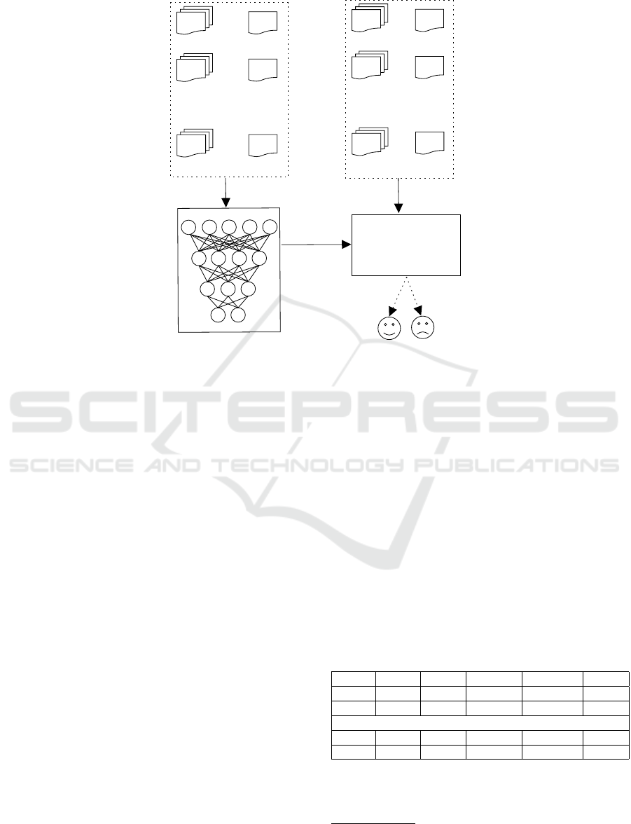
Our aim is to create a sentiment forecasting
model that depends on supervised learning. Its
role is to classify the past content of a user ac-
cording to a specific topic. We consider the train-
ing set D = {(c
1
,t
e
1
,s
1
),...,(c
`
,t
e
`
,s
`
)}, and F =
{(c
`+1
,t
e
`+1
,s
`+1
),...,(c
p
,t
e
p
,s
p
)} is the set of test,
where (c
k
,t
e
k
) represents the input sample of the
model, s
k
represents its output, and c
k
is the past con-
tent of user u
e
k
who wrote tweet e
k
about topic t
e
k
and
its sentiment s
k
(see figure 1).
3.2 Model Description
3.2.1 Embedded Layer
As aforementioned, the input of our model is a set of
past tweets from a user,as well as a topic, to predict
its sentiment polarity.
First, we have to pass the inputs to a layer called the
embedding layer. Its role is to convert words to real
values where each passed tweet becomes a matrix of
real numbers, and so is for the topic. This conver-
sion is based on a dictionary, named word embedding,
where each word is represented by a vector of real
numbers. In general, it is generated from techniques
that take a set of textual documents in order to find
a numerical representation of words where the dis-
tances between them are semantic ones. Eventually,
we have multiple inputs: c
k
is a set of past tweets rep-
resented by matrices where one tweet is represented
as c
k
j
∈ R
v×d
and the topic t
e
k
is represented in the
same way as c
k
j
. It is worth mentioning that we use
the ”zero-padding” technique in order to obtain the
same word count dimension v of all tweets and topics.
Then, the tweets will be treated by an LSTM-based
model.
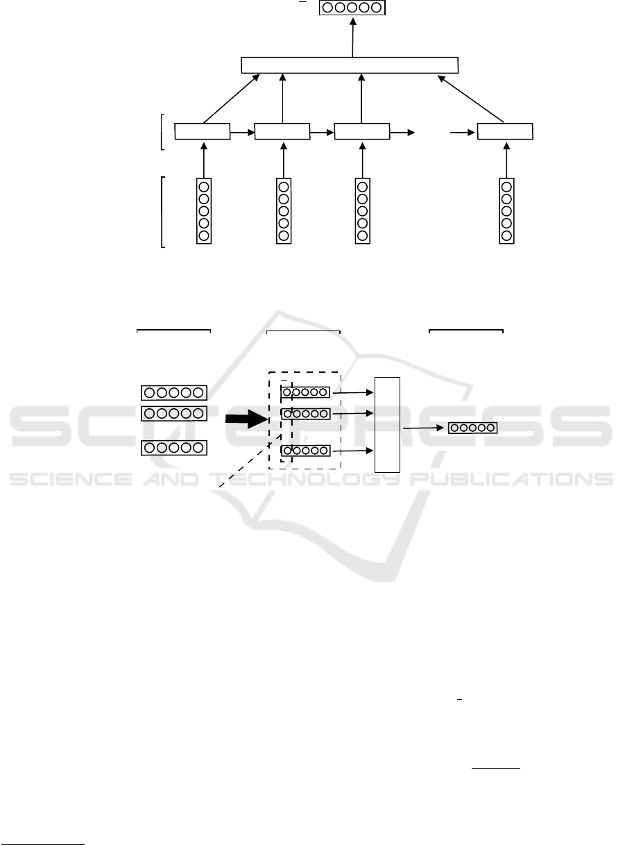
3.2.2 Sub-model based on LSTM
To extract the semantic meaning for tweets(Zhang
et al., 2016), we used the LSTM layer, which is an
improvement of the RNN operation designed to man-
age the input in the sequence form, to obtain either a
prediction of the next element of it, or to encode in
order to have a new encoded sequence. If we pass a
set of tweet words c
k
j
= [x
1
,...,x
v
] as a sequence, each
one is the input of an RNN-cell and at each step t the
hidden state h
t
is calculated as follows(Elman, 1990):
h
t
= f (W
h
x
t
+Uh
t−1
+ b
h
) (1)
The limit of RNNs resides in the exploding and
Vanishing gradient(Hochreiter et al., 2001). LSTM
overcomes this problem and provides larger mem-
ory to store more past data. The hidden state h
t
of LSTM cell is calculated as follows(Gers et al.,
1999)(Hochreiter and Schmidhuber, 1997):
i
t
= σ(W
i
x
t
+U
i
h
t−1
+ b
i
) (2)
f
t
= σ(W
f
x
t
+U
f
h
t−1
+ b
f
) (3)
o
t
= σ(W
o
x
t
+U
o
h
t−1
+ b
o
) (4)
g
t
= σ(W
g
x
t
+U
g
h
t−1
+ b
g
) (5)
c
t
= f
t
◦ c
t−1
+ i
t
◦ g
t
(6)
h
t
= o
t
◦ tanh(c
t
) (7)
where i
t
, f
t
and o
t
are respectively the input, forget
and output gates, σ and tanh are the sigmoid and hy-
perbolic tangent functions, and ◦ is the element-wise
product operator. After getting the vector of different
hidden states of each word h
j
= [h
1
,...,h
v
], we feed-
forward it to the average pooling layer, which simply
averages the elements of h
j
(see figure 2). This model
is applied in a distributed manner to each past tweet,
and it is applied also to the input topic. Before pass-
ing to the convolution layer, an averaging operation is
done between the output generated by the precedent
model of each past tweet and that of the topic. It is
represented by F
j
, and it is the feature vector gener-
ated between c
k
j
and the topic t
e
k
.
3.2.3 Sub-model based on CNN-LSTM
A convolution layer is applied on the output of the
precedent layer. It is based on the one proposed by
(Kim, 2014). We apply one filter of size h for each
region size. For example, to produce a map feature
z = [z
1
,...,z
Q−h+1
] , a filter W ∈ R
h×d
is multiplied
by the n-gram tweet sequences, and an element of z is
calculated as follows:
z
n
= f (W.c
k
j
n:n+h
1
−1
+ b) (8)
where b ∈ R is a bias value and f (x) is a non-
linear function such as the ReLU function. Generally,
the layer that follows the convolution layer is max-
pooling, but we choose to replace it with the LSTM
layer, in order to improve the performance and the
time complexity (Hassan and Mahmood, 2018)(see
figure 3).
WEBIST 2021 - 17th International Conference on Web Information Systems and Technologies
244

...
C
1
C
2
C
`
t
e
1
t
e
2
t
e
`
Training set
...
C
`+1
C
`+2
C
p
t
e
`+1
t
e
`+2
t
e
p
Test set
Classifier
Training step
Figure 1: Overview of our approach.
3.2.4 Classification Layer
Finally, the output of the CNN-LSTM sub-model
goes through the classification layer. It is a sigmoid
activation function and its role is to compute the pre-
dicted probabilities of both categories (positive or
negative sentiments). We can see the overall archi-
tecture of the approach in figure 4.
4 EXPERIMENTS
4.1 Data Collection
In this work, we need a specific collection of users
who have posted tweets on different topics and their
polarities, as well as the past tweets of each user.
The SemEval-2017 (Rosenthal et al., 2019a) data
and specifically the sub-task B data (classification
of tweets according to the 2 polarities, positive and
negative). In fact, it is an appropriate collection to
create our own one. The tweets collection is com-
posed of a training set, which was collected from July
to December 2015 (the English tweets collection of
SemEval-2016 (Nakov et al., 2019) and also some of
SemEval-2015 (Rosenthal et al., 2019b)), and the test
set, which was collected from December 2016 to Jan-
uary 2017. Several categories of tweets topics can be
distinguished, such as public personalities, athletes,
artists, books, social phenomena, movies, etc. For
each tweet in the collection of two sets, we collect
the past tweets of its author, using python package
1
.
Unfortunately, after the collection of past tweets, we
delete tweets for the following reasons:
• Unavailable authors (deleted or secure account)
• Authors who only have a number of past tweets
below 30 (the maximum number is 300)
• An author who has written more than once on the
same topic. In this case we just keep the first tweet
Table 1 shows the statistics before and after the col-
lection of past tweets.
Table 1: Statistic collection.
Topic User Positive Negative Total
Train 373 - 14,951 4,013 18964
Test 125 - 2,463 3,722 6185
After past tweets collection
Train 348 10132 8104 2092 10196
Test 115 2476 788 1710 2498
1
https://github.com/Jefferson-Henrique/GetOldTweets-
python
Prediction Sentiment Polarity using Past Textual Content and CNN-LSTM Neural Networks
245

LSTM Cell
LSTM Cell
...
LSTM Cell
Input
Sequence
LSTM
Layer
Average Pooling
...
x
j
1
x
j
2
x
j
3
x
j
v
h
j
1
h
j
2
h
j
3
h
j
v
h
j
C
k
j
...
LSTM Cell
Figure 2: LSTM Sub-model.
...
...
Convolution results
with m filters
(Q −h + 1) × m
F
1
F
2
F
Q
LSTM Layer
...
Map feature vector
Input
Output
Figure 3: CNN-LSTM Sub-model.
4.2 Tweet Pre-processing
Tweets must go through the pre-processing stage be-
fore being fed to the learning models. To do this, we
apply the following different steps:
• Remove URLs.
• Replace emojis by their short name such as
<smile>, <laughing>, <worried>, etc. (using
python package
2
)
• Convert tweet text to all lowercase letters.
4.3 Pre-trained Word Embeddings
We choose the unsupervised word embeddings model
of Datasories(Baziotis et al., 2017) work, in order to
initialize the word vectors. It is generated from a
large number of tweets using Glove(Pennington et al.,
2
https://pypi.org/project/emoji/
2014). Its availability and performance allows us to
rely on it.
4.4 Evaluation Measures
The performance is evaluated using average recall,
F1- score and accuracy. These metrics have been used
by SemEval participants. They are defined as follows:
R =
1
2
(R
P
+ R
N
)
(9)
where R
P
and R
N
represent the positive and negative
recalls, respectively.
F
PN
1
=
F
P
1
+ F
N
1
2
(10)
where F
P
1
and F
N
1
represent the positive and negative
F1-score, respectively.
Finally, accuracy is simply the ratio between the
number of observations correctly assigned to the total
number.
WEBIST 2021 - 17th International Conference on Web Information Systems and Technologies
246

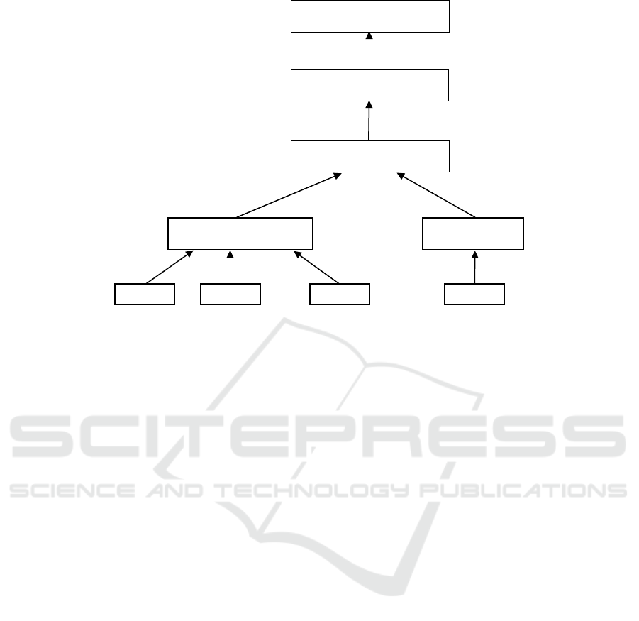
Shared LSTM Sub-Model
Tweet 1 Tweet 2
Tweet Q
...
LSTM Sub-Model
Topic
Average layer
CNN-LSTM Sub-Model
Classification layer
Figure 4: Architecture of proposed approach.
Since the dataset is divided into several topics, we
calculate the measures individually for each topic and
then average the results across the topics. As a result,
the results obtained are named as follows: AvgRecall,
AvgFscore and AvgAcc.
4.5 Optimization
We randomly divide the training set into two subsets,
the division is made by topics whith 20% for the val-
idation set and the rest for the training set. After
a validation of parameters, we used an LSTM layer
with hidden state dimension of size 32 for LSTM sub-
model. For the CNN-LSTM sub-model, a convolu-
tion layer is considered with a filter number of 256
and a kernel size equal to 1 (chosen after a validation
step with several numbers when the past tweets num-
ber is set at 10), followed by an LSTM layer of size
128.
Finally, to reduce the model over-fitting, we add some
dropout layers: the first layer is after the embedding
layers, one other before the average layer, one other
between the CNN and LSTM layers in the CNN-
LSTM sub-model and last one before the classifica-
tion layer. In addition, we have use the L2 vector
norms for the regularization of weights for certain lay-
ers. A validation of the past tweets number parameter
Q is done after a model evaluation on multiple num-
bers ([15,10,30,50,100,150,200,250,300]) on the val-
idation set. Table 3 contains the results of the model
experimented on the test set.
For sentiment-intensity-based approach (Bel-
hareth and Latiri, 2019), we follow the cross-
validation technique by setting the number of past
tweets to 10. then, validate the validation of the past
tweets number Q by the same technique (we also used
the cosine similarity measure for ranking the past
tweets). We also use the Principal Component Analy-
sis (PCA)(Abdi and Williams, 2010) technique to re-
duce data dimensions by extracting important infor-
mation in order to improve the performance of classi-
fiers.
4.6 Results and Discussion
Table 3 shows the results of different models exper-
imented on the test set. For the sentiment-intensity-
based approach, the PCA technique improves the per-
formance of all classifiers except the Linear SVM
classifier. We can note that the classifier naive bayes
with PCA is the best model for this approach. On
the other hand, our approach outperforms all compari-
son models, and outperforms the best models by more
than 4% for the AvgRecall metric, by about 5% for the
AvgFscore metric and by around 6% for the AvgAcc
metric.
In addition, we notice that the number of past
tweets chosen for the different classifiers as well as
our approach are divergent, and this requires us to do
a deep analysis in order to understand its effect.
Furthermore, a comparison with a model that di-
rectly processes the tweets that carry the sentiment
without the past tweets is recommended in order to
evaluate the utility of processing only the past tweets.
Prediction Sentiment Polarity using Past Textual Content and CNN-LSTM Neural Networks
247

Table 2: Some observations of SemEval-2017 collection.
Id Topic: t
e
k
Polarity: s
k
Text: e
k
802377144638709760 social security negative history is like your social
Security number. long, use-
less, but needed.
805705353493155840 brexit positive @pimpmytweeting Happy
birthday have a great day
and drink a toast Brexit
805659700104691713 abortion negative I pray that you are against
abortion, and political can-
didates who allow/promote
abortion, to the same de-
gree UR against the death
penalty.
802351474005209088 wall on the mexican border positive @BIZPACReview This is
great news. For a Mexican
effort to build a parallel wall
on their side of the border
too.
Table 3: Results of different comparison models and our approach according to specified metrics.
Methode Past tweets number: Q AvgRecall AvgFscore AvgAcc
Sentiment-intensity-based approach
Naive Bayes
Without PCA 30 0.570414 0.541824 0.704695
With PCA 100 0.594532 0.565484 0.717732
Logistic Regression
Without PCA 300 0.575018 0.502351 0.605860
With PCA 300 0.593699 0.506071 0.614399
Random Forest
Without PCA 10 0.459768 0.356416 0.454842
With PCA 20 0.539360 0.418966 0.515915
Linear SVM
Without PCA 300 0.297630 0.319390 0.413075
With PCA 10 0.288931 0.318957 0.412645
RBF SVM
Without PCA 20 0.567220 0.481756 0.573595
With PCA 30 0.592770 0.493887 0.581992
Our approach 10 0.639172 0.612123 0.774180
5 CONCLUSION
In this paper, a sentiment prediction approach is pro-
posed, depending uniquely on users’ past tweets, and
the objective is to predict their sentiment polarities
on a specific topic. To do so, we have created a col-
lection from the SemeEval-2017 collection. Our ap-
proach depends on the LSTM and CNN architectures
performs better than the different suggested compari-
son models. In the end, it is necessary, first, to create
a collection that is balanced at the polarity class level
and which contains more than two classes to better
test the approach and, second, to use other feature ex-
traction techniques to improve the performance.
REFERENCES
Abdi, H. and Williams, L. J. (2010). Principal component
analysis. Wiley interdisciplinary reviews: computa-
tional statistics, 2(4):433–459.
Asur, S. and Huberman, B. A. (2010). Predicting the future
with social media. In 2010 IEEE/WIC/ACM interna-
tional conference on web intelligence and intelligent
agent technology, volume 1, pages 492–499. IEEE.
Baziotis, C., Pelekis, N., and Doulkeridis, C. (2017). Datas-
tories at semeval-2017 task 4: Deep lstm with atten-
tion for message-level and topic-based sentiment anal-
ysis. In Proceedings of the 11th international work-
shop on semantic evaluation (SemEval-2017), pages
747–754.
Belhareth, Y. and Latiri, C. (2019). Microblog sentiment
prediction based on user past content. In WEBIST,
pages 250–256.
WEBIST 2021 - 17th International Conference on Web Information Systems and Technologies
248

Cliche, M. (2017). Bb twtr at semeval-2017 task 4: Twitter
sentiment analysis with cnns and lstms. arXiv preprint
arXiv:1704.06125.
Conde-Cespedes, P., Chavando, J., and Deberry, E. (2018).
Detection of suspicious accounts on twitter using
word2vec and sentiment analysis. In International
Conference on Multimedia and Network Information
System, pages 362–371. Springer.
Djaballah, K. A., Boukhalfa, K., and Boussaid, O.
(2019). Sentiment analysis of twitter messages us-
ing word2vec by weighted average. In 2019 Sixth In-
ternational Conference on Social Networks Analysis,
Management and Security (SNAMS), pages 223–228.
IEEE.
Elman, J. L. (1990). Finding structure in time. Cognitive
science, 14(2):179–211.
Gers, F. A., Schmidhuber, J., and Cummins, F. (1999).
Learning to forget: Continual prediction with lstm.
Hassan, A. and Mahmood, A. (2018). Convolutional recur-
rent deep learning model for sentence classification.
Ieee Access, 6:13949–13957.
Hochreiter, S., Bengio, Y., Frasconi, P., Schmidhuber, J.,
et al. (2001). Gradient flow in recurrent nets: the dif-
ficulty of learning long-term dependencies.
Hochreiter, S. and Schmidhuber, J. (1997). Long short-term
memory. Neural computation, 9(8):1735–1780.
Jim
´
enez-Zafra, S. M., Montejo-R
´
aez, A., Mart
´
ın-Valdivia,
M. T., and Lopez, L. A. U. (2017). Sinai at semeval-
2017 task 4: User based classification. In Proceedings
of the 11th International Workshop on Semantic Eval-
uation (SemEval-2017), pages 634–639.
Kim, Y. (2014). Convolutional neural networks for sentence
classification. arXiv preprint arXiv:1408.5882.
Kolovou, A., Kokkinos, F., Fergadis, A., Papalampidi, P.,
Iosif, E., Malandrakis, N., Palogiannidi, E., Papageor-
giou, H., Narayanan, S., and Potamianos, A. (2017).
Tweester at semeval-2017 task 4: Fusion of semantic-
affective and pairwise classification models for sen-
timent analysis in twitter. In Proceedings of the
11th International Workshop on Semantic Evaluation
(SemEval-2017), pages 675–682.
M
¨
uller, S., Huonder, T., Deriu, J. M., and Cieliebak, M.
(2017). Topicthunder at semeval-2017 task 4: Senti-
ment classification using a convolutional neural net-
work with distant supervision. In Proceedings of the
11th International Workshop on Semantic Evaluation
(SemEval-2017), pages 766–770.
Nakov, P., Ritter, A., Rosenthal, S., Sebastiani, F., and Stoy-
anov, V. (2019). Semeval-2016 task 4: Sentiment
analysis in twitter. arXiv preprint arXiv:1912.01973.
Nguyen, L. T., Wu, P., Chan, W., Peng, W., and Zhang,
Y. (2012). Predicting collective sentiment dynamics
from time-series social media. In Proceedings of the
First International Workshop on Issues of Sentiment
Discovery and Opinion Mining, WISDOM ’12, New
York, NY, USA. Association for Computing Machin-
ery.
Nguyen, T. H., Shirai, K., and Velcin, J. (2015). Sentiment
analysis on social media for stock movement predic-
tion. Expert Systems with Applications, 42(24):9603
– 9611.
Pennington, J., Socher, R., and Manning, C. D. (2014).
Glove: Global vectors for word representation. In
Proceedings of the 2014 conference on empirical
methods in natural language processing (EMNLP),
pages 1532–1543.
Rosenthal, S., Farra, N., and Nakov, P. (2019a). Semeval-
2017 task 4: Sentiment analysis in twitter. arXiv
preprint arXiv:1912.00741.
Rosenthal, S., Mohammad, S. M., Nakov, P., Ritter, A., Kir-
itchenko, S., and Stoyanov, V. (2019b). Semeval-2015
task 10: Sentiment analysis in twitter. arXiv preprint
arXiv:1912.02387.
Si, J., Mukherjee, A., Liu, B., Li, Q., Li, H., and Deng,
X. (2013). Exploiting topic based twitter sentiment
for stock prediction. In Proceedings of the 51st An-
nual Meeting of the Association for Computational
Linguistics (Volume 2: Short Papers), pages 24–29.
Tumasjan, A., Sprenger, T. O., Sandner, P. G., and Welpe,
I. M. (2010). Predicting elections with twitter: What
140 characters reveal about political sentiment. In
Fourth international AAAI conference on weblogs and
social media.
Wilson, T. D. and Gilbert, D. T. (2003). Affective forecast-
ing.
Yoo, S., Song, J., and Jeong, O. (2018). Social media con-
tents based sentiment analysis and prediction system.
Expert Systems with Applications, 105:102 – 111.
Zhang, R., Lee, H., and Radev, D. R. (2016). Dependency
sensitive convolutional neural networks for modeling
sentences and documents. CoRR, abs/1611.02361.
Zhou, C., Wang, J., and Zhang, X. (2019). Ynu-hpcc at
semeval-2019 task 6: Identifying and categorising of-
fensive language on twitter. In Proceedings of the
13th International Workshop on Semantic Evaluation,
pages 812–817.
Prediction Sentiment Polarity using Past Textual Content and CNN-LSTM Neural Networks
249